Quadratic Residues Definition : The numbers 0 2 , 1 2 , 2 2 , . . . , - - PowerPoint PPT Presentation

SLIDE 1

Introduction to Number Theory 2

c Eli Biham - May 3, 2005 348 Introduction to Number Theory 2 (12)

Quadratic Residues

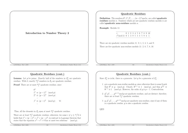
Definition: The numbers 02, 12, 22, . . . , (n−1)2 mod n, are called quadratic residues modulo n. Numbers which are not quadratic residues modulo n are called quadratic non-residues modulo n. Example: Modulo 11: i 0 1 2 3 4 5 6 7 8 9 10 i2 mod 11 0 1 4 9 5 3 3 5 9 4 1 There are six quadratic residues modulo 11: 0, 1, 3, 4, 5, and 9. There are five quadratic non-residues modulo 11: 2, 6, 7, 8, 10.

c Eli Biham - May 3, 2005 349 Introduction to Number Theory 2 (12)

Quadratic Residues (cont.)

Lemma: Let p be prime. Exactly half of the numbers in Z∗

p are quadratic

• residues. With 0, exactly p+1

2 numbers in Zp are quadratic residues.

Proof: There are at most p+1

2 quadratic residues, since

02 12 ≡ (p − 1)2 (mod p) 22 ≡ (p − 2)2 (mod p) . . . i2 ≡ (p − i)2 (mod p) ∀i . . . Thus, all the elements in Zp span at most p+1

2 quadratic residues.

There are at least p+1

2

quadratic residues, otherwise, for some i = j ≤ p−1

/ 2 it

holds that i2 = (p − i)2 = j2 = (p − j)2, in contrast to Lagrange theorem that states that the equation x2 − i2 = 0 has at most two solutions (mod p).

c Eli Biham - May 3, 2005 350 Introduction to Number Theory 2 (12)

Quadratic Residues (cont.)

Since Z∗

p is cyclic, there is a generator. Let g be a generator of Z∗ p.

• 1. g is a quadratic non-residue modulo p, since otherwise there is some b such

that b2 ≡ g (mod p). Clearly, bp−1 ≡ 1 (mod p), and thus g

p−1 2

≡ bp−1 ≡ 1 (mod p). However, the order of g is p − 1. Contradiction.

• 2. g2, g4, . . . , g(p−1) mod p are quadratic residues, and are distinct, therefore,

there are at least p−1

2 quadratic residues.

• 3. g, g3, g5, . . . , g(p−2) mod p are quadratic non-residues, since if any of them

is a quadratic residue, g is also a quadratic residue. QED

c Eli Biham - May 3, 2005 351 Introduction to Number Theory 2 (12)

SLIDE 2

Euler’s Criterion

Theorem: Let p = 2 be a prime, and let a ∈ Z∗

• p. Then, a is a quadratic

residue modulo p iff a

p−1 2 ≡ 1

(mod p). Proof: (⇒) If a is a quadratic residue, there is some b such that a ≡ b2 (mod p). Thus, a

p−1 2 ≡ (b2) p−1 2 ≡ bp−1 ≡ 1

(mod p).

c Eli Biham - May 3, 2005 352 Introduction to Number Theory 2 (12)

Euler’s Criterion (cont.)

(⇐) If a is a quadratic non-residue: For any r there is a unique s such that rs ≡ a (mod p), i.e., s = ar−1, and there is no r∗ = r such that s = ar∗−1. Since a is a quadratic non-residue, r ≡ s (mod p). Thus, the numbers 1, 2, 3, . . . , p − 1 are divided into p−1

2 distinct pairs (r1, s1),

(r2, s2), . . . , (rp−1

2 , sp−1 2 ), such that risi = a, and we get

a

p−1 2

≡ r1s1r2s2 . . . rp−1

2 sp−1 2 ≡

≡ 1 · 2 · . . . · (p − 1) ≡ −1 (mod p) by Wilson’s theorem. QED

c Eli Biham - May 3, 2005 353 Introduction to Number Theory 2 (12)

Quadratic Residues Modulo n = pq

Let p and q be large primes and let n = pq (as in RSA). Theorem: Let m ∈ Z∗

• n. If m is a quadratic residue modulo n, then m has

exactly four square roots modulo n in Z∗

n.

Proof: Assume α2 ≡ m (mod n). Then gcd(m, n) = 1 ⇒ gcd(α2, n) = 1 ⇒ gcd(α, n) = 1 ⇒ α ∈ Z∗

n.

and since m ≡ α2 (mod n) then m ≡ α2 (mod p) m ≡ α2 (mod q) m has two square roots modulo p (α mod p and −α mod p) and two square roots modulo q (α mod q and −α mod q).

c Eli Biham - May 3, 2005 354 Introduction to Number Theory 2 (12)

Quadratic Residues Modulo n = pq (cont.)

Look at the systems of equations x ≡ ±α (mod p) x ≡ ±α (mod q) which represent four systems (one of each possible choice of ±). Each system has an unique solution modulo n which satisfies x2 ≡ m (mod p) x2 ≡ m (mod q) and thus satisfies x2 ≡ m (mod n) All the four solutions are roots of m modulo n. These are all the roots. Otherwise there must be more than two roots either modulo p or modulo q. QED

c Eli Biham - May 3, 2005 355 Introduction to Number Theory 2 (12)

SLIDE 3

Quadratic Residues Modulo n = pq (cont.)

Conclusion: Exactly a quarter of the numbers in Z∗

n are quadratic residues

modulo n.

c Eli Biham - May 3, 2005 356 Introduction to Number Theory 2 (12)

Legendre’s Symbol

Definition: Let p be a prime such that p |a. Legendre’s symbol of a

• ver p is

   a

p

    ∆

=

    

+1, if a is a quadratic residue modulo p; −1, if a is a quadratic non-residue modulo p. By Euler:

   a

p

    ≡ a p−1 2

(mod p).

c Eli Biham - May 3, 2005 357 Introduction to Number Theory 2 (12)

Legendre’s Symbol (cont.)

Properties of Legendre’s symbol:

• 1. a ≡ a′

(mod p) ⇒

• a

p

• =
• a′

p

• .

2.

• 1

p

• =
• c2

p

• = 1

∀c. 3.

• −1

p

• =

    

1, if p = 4k + 1; −1, if p = 4k + 3. Proof:

   −1

p

    ≡ (−1) p−1 2

(mod p) ≡

      

(−1)

4k+1−1 2

≡ (−1)2k ≡ 1, if p = 4k + 1; (−1)

4k+3−1 2

≡ (−1)2k+1 ≡ −1, if p = 4k + 3.

c Eli Biham - May 3, 2005 358 Introduction to Number Theory 2 (12)

Legendre’s Symbol (cont.)

4.

• 2

p

• = (−1)

p2−1 8 .

(given without a proof). 5.

• ab

p

• =
• a

p b p

• .

Proof: Let g be a generator modulo p. Then, ∃i, a ≡ gi (mod p) and ∃j, b ≡ gj (mod p). a is a quadratic residue iff i is even, b is a quadratic residue iff j is even, and ab is a quadratic residue iff i + j is even. Thus, by Euler:

   ab

p

    ≡ (−1)i+j ≡ (−1)i(−1)j ≡    a

p

       b

p

   

(mod p).

c Eli Biham - May 3, 2005 359 Introduction to Number Theory 2 (12)

SLIDE 4

Legendre’s Symbol (cont.)

• 6. The reciprocity law: if p = q are both odd primes then

   p

q

    = (−1) p−1 2 q−1 2    q

p

    .

(given without a proof).

c Eli Biham - May 3, 2005 360 Introduction to Number Theory 2 (12)

Jacobi’s Symbol

Jacobi’s symbol is a generalization of Legendre’s symbol to composite numbers. Definition: Let n be odd, and let p1, p2, . . . , pk be the prime factors of n (not necessarily distinct) such that n = p1p2 · · · pk. Let a be coprime to n. Jacobi’s symbol of a over n is

 a

n

  ∆

=

    a

p1

        a

p2

    · · ·     a

pk

    .

In particular, for n = pq

 a

n

  =     a

pq

    =    a

p

       a

q

    .

c Eli Biham - May 3, 2005 361 Introduction to Number Theory 2 (12)

Jacobi’s Symbol (cont.)

Remarks:

• 1. a ∈ Z∗

n is a quadratic residue modulo n iff the Legendre’s symbols over

all the prime factors are 1.

• 2. When Jacobi’s symbol is 1, a is not necessarily a quadratic residue.
• 3. When Jacobi’s symbol is -1, a is necessarily a quadratic non-residue.

c Eli Biham - May 3, 2005 362 Introduction to Number Theory 2 (12)

Jacobi’s Symbol (cont.)

Properties of Jacobi’s symbol: Let m and n be integers, and let a and b be coprime to m and n. Assume that n is odd and that the factorization of n is n = p1p2 · · · pk.

• 1. a ≡ b

(mod n) ⇒

a

n

• =

b

n

• .

2.

1

n

• = 1

∀n (1 is a quadratic residue modulo any n). 3.

−1

n

• = (−1)

n−1 2 .

Proof: n = p1p2 · · · pk = ((p1 − 1) + 1)((p2 − 1) + 1) · · · ((pk − 1) + 1)

• pening parentheses:

=

• S⊆{1,2,...,k}
• i∈S(pi − 1)

c Eli Biham - May 3, 2005 363 Introduction to Number Theory 2 (12)

SLIDE 5

Jacobi’s Symbol (cont.)

=

       

• S⊆{1,2,...,k}

|S|≥2

• i∈S(pi − 1)

        +

• i∈{1,2,...,k}(pi − 1) + 1

= [(p1 − 1)(p2 − 1) · · · (pk − 1) + . . .] + (p1 − 1) + (p2 − 1) + . . . + (pk − 1) + 1 where all the terms with |S| ≥ 2 (in the brackets) are multiples of four, and all the pi − 1 are even. Thus, n − 1 2 ≡ (p1 − 1) 2 + (p2 − 1) 2 + . . . + (pk − 1) 2 (mod 2), and

  −1

n

   =    −1

p1

       −1

p2

    · · ·    −1

pk

   

= (−1)(p1−1)/2(−1)(p2−1)/2 · · · (−1)(pk−1)/2 = (−1)(p1−1)/2+(p2−1)/2+...+(pk−1)/2 = (−1)(n−1)/2.

c Eli Biham - May 3, 2005 364 Introduction to Number Theory 2 (12)

Jacobi’s Symbol (cont.)

4.

2

n

• = (−1)

n2−1 8 .

Proof: We saw that

• 2

p

• = (−1)

p2−1 8 , thus:   2

n

   =     2

p1

        2

p2

    · · ·     2

pk

    = (−1) p2 1−1 8 + p2 2−1 8 +···+ p2 k−1 8

It remains to show that n2 − 1 8 ≡ p2

1 − 1

8 + p2

2 − 1

8 + · · · + p2

k − 1

8 (mod 2) q2

1q2 2 = (1 + (q2 1 − 1))(1 + (q2 2 − 1))

= 1 + (q2

1 − 1) + (q2 2 − 1) + (q2 1 − 1)(q2 2 − 1)

But 8|(q2

1 − 1) and 8|(q2 2 − 1), thus 64|(q2 1 − 1)(q2 2 − 1). Therefore,

q2

1q2 2 ≡ 1 + (q2 1 − 1) + (q2 2 − 1)

(mod 16)

c Eli Biham - May 3, 2005 365 Introduction to Number Theory 2 (12)

Jacobi’s Symbol (cont.)

And, q2

1q2 2q2 3 ≡ (1 + (q2 1 − 1))(1 + (q2 2 − 1))(1 + (q2 3 − 1))

(mod 16) ≡ 1 + (q2

1 − 1) + (q2 2 − 1) + (q2 3 − 1)

(mod 16) etc., thus, n2 ≡ 1 + (q2

1 − 1) + (q2 2 − 1) + · · · + (q2 k − 1)

(mod 16) n2 − 1 8 ≡ p2

1 − 1

8 + p2

2 − 1

8 + · · · + p2

k − 1

8 (mod 2)

c Eli Biham - May 3, 2005 366 Introduction to Number Theory 2 (12)

Jacobi’s Symbol (cont.)

• 5. The first multiplication property:

a

mn

• =

a

m

a

n

• .

(if a is coprime to mn it is coprime to m and to n; the rest is derived directly from the definition).

• 6. The second multiplication property:

ab

n

• =

a

n

b

n

• .

(if ab is coprime to n, the both a and b are coprime to n; the rest is derived since this property holds for Legendre’s symbol).

c Eli Biham - May 3, 2005 367 Introduction to Number Theory 2 (12)

SLIDE 6

Jacobi’s Symbol (cont.)

• 7. The reciprocity law: if m, n are coprime and odd then

  n

m

  = (−1) m−1 2 n−1 2  m

n

  .

Proof: First assume that m = q is a prime, thus,

   n

q

    =    p1

q

       p2

q

    · · ·    pk

q

    .

By the reciprocity law of Legendre’s symbol we know that

   pi

q

    = (−1) pi−1 2 q−1 2     q

pi

    .

Thus,

   n

q

    = (−1) q−1 2 (p1−1 2 +...+pk−1 2 )     q

p1

        q

p2

    · · ·     q

pk

   

• ( q

n)

.

c Eli Biham - May 3, 2005 368 Introduction to Number Theory 2 (12)

Jacobi’s Symbol (cont.)

We saw in property 3 that, n − 1 2 ≡ (p1 − 1) 2 + (p2 − 1) 2 + . . . + (pk − 1) 2 (mod 2), thus,

   n

q

    = (−1) q−1 2 n−1 2  q

n

  .

Now for any odd m:

  n

m

  =     n

q1

        n

q2

    · · ·    n

qℓ

   

=

 q1

n

   q2

n

  · · ·  qℓ

n

  (−1) n−1 2 (q1−1 2 +...+qℓ−1 2 )

= (−1)

m−1 2 n−1 2  m

n

 

QED

c Eli Biham - May 3, 2005 369 Introduction to Number Theory 2 (12)

Jacobi’s Symbol (cont.)

Application of Jacobi’s Symbol: Using the properties of Jacobi’s symbol, it is easy to calculate Legendre’s sym- bols in polynomial time. Example:

  117

271

   = ↑

7

+1 ·

  271

117

   = ↑

1

   37

117

   = ↑

7

  117

37

   = ↑

1

   6

37

  

=

↑

6

   2

37

      3

37

   = ↑

4

(−1)

   3

37

   = ↑

7

(−1)(+1)

  37

3

  

=

↑

1

(−1)(+1)

  1

3

   = ↑

2

(−1)(+1)1 = −1 271 is prime, therefore

117

271

• can also be computed by:

  117

271

   ≡ 117 271−1 2

≡ 117135 ≡ −1 (mod 271).

c Eli Biham - May 3, 2005 370 Introduction to Number Theory 2 (12)

Jacobi’s Symbol (cont.)

Complexity: The only required arithmetic operations are modular reductions and division by powers of two. Clearly, a division (rule 6) reduces the “numerator” by a factor of two. A modular reduction (using rule 7 and then rule 1), reduces the number by at least two: as if a > b then a = qb + r ≥ b + r > r + r, thus r < a/2, i.e, a mod b < a/2. Therefore, at most O(log n) modular reductions/divisions are performed, each

• f which takes O((log n)2) time. This shows that the complexity is O((log n)3),

which is polynomial in log n. A more precise analysis of this algorithm shows that the complexity can be reduced to O((log n)2).

c Eli Biham - May 3, 2005 371 Introduction to Number Theory 2 (12)