Quasi-Statistical Manifolds and Geometry of Affine Distributions - - PowerPoint PPT Presentation

quasi statistical manifolds and geometry of affine
SMART_READER_LITE
LIVE PREVIEW

Quasi-Statistical Manifolds and Geometry of Affine Distributions - - PowerPoint PPT Presentation

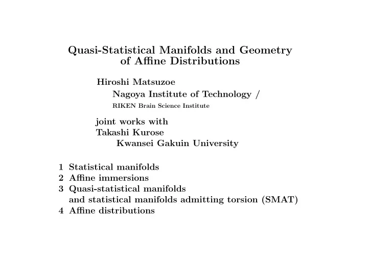
Quasi-Statistical Manifolds and Geometry of Affine Distributions Hiroshi Matsuzoe Nagoya Institute of Technology / RIKEN Brain Science Institute joint works with Takashi Kurose Kwansei Gakuin University 1 Statistical manifolds 2 Affine


slide-1
SLIDE 1

Quasi-Statistical Manifolds and Geometry

  • f Affine Distributions

Hiroshi Matsuzoe Nagoya Institute of Technology /

RIKEN Brain Science Institute

joint works with Takashi Kurose Kwansei Gakuin University 1 Statistical manifolds 2 Affine immersions 3 Quasi-statistical manifolds and statistical manifolds admitting torsion (SMAT) 4 Affine distributions

slide-2
SLIDE 2

Geometry of Affine Distributions

2

1 Statistical manifolds

M : a manifold (an open domain in Rn) h : a (semi-) Riemannian metric on M ∇ : an affine connection on M

✓ ✏

Definition 1.1 (Kurose) We say that the triplet (M, ∇, h) is a statistical manifold

def

⇐ ⇒ (∇Xh)(Y, Z) = (∇Y h)(X, Z).

✒ ✑

C(X, Y, Z) := (∇Xh)(Y, Z), the cubic form, the skewness tensor field

✓ ✏

Definition 1.2 ∇∗: the dual connection of ∇ with respect to h

def

⇐ ⇒ Xh(Y, Z) = h(∇∗

XY, Z) + h(Y, ∇XZ).

✒ ✑

(M, ∇∗, h): the dual statistical manifold of (M, ∇, h).

✓ ✏

Remark 1.3 (Original definition by S.L. Lauritzen) (M, g) : a Riemannian manifold C : a totally symmetric (0, 3)-tensor field We call the triplet (M, g, C) a statistical manifold.

✒ ✑

slide-3
SLIDE 3

Geometry of Affine Distributions

3

Example 1.4 (Normal distributions) ( l(x; ξ) = log p(x, ξ) ) M = {p(x; ξ) | ξ = (ξ1, ξ2) = (µ, σ), p(x; ξ) = 1 √ 2π(ξ2)2 exp [ −(x − ξ1)2 2(ξ2)2 ] = 1 √ 2πσ2 exp [ −(x − µ)2 2σ2 ] } We regard that M is a manifold with local coordinates (µ, σ). gij = ∫ ∞

−∞

( ∂ ∂ξi log p(x, ξ) ) ( ∂ ∂ξj log p(x, ξ) ) p(x, ξ)dx = E [ ∂l ∂ξi ∂l ∂ξj ] ( g = − 1 σ2 ( 1 0 0 2 )) the Fisher information Cijk = E [ ∂l ∂ξi ∂l ∂ξj ∂l ∂ξk ] the skewness or the cubic form Γij,k = E [ ∂2l ∂ξi∂ξj ∂l ∂ξk ] = Γ(0)

ij,k − 1

2Cijk ( ∇(0): the Levi-Civita connection w.r.t. g ) Γ∗

ij,k = E

[ ∂2l ∂ξi∂ξj ∂l ∂ξk + ∂l ∂ξi ∂l ∂ξj ∂l ∂ξk ] = Γ(0)

ij,k + 1

2Cijk (M, ∇, g) and (M, ∇∗, g) are statistical manifolds.

slide-4
SLIDE 4

Geometry of Affine Distributions

4

2 Affine immersions

f : M → Rn+1: an immersion ξ: a local vector field along f

✓ ✏

Definition 2.1 {f, ξ} : M → Rn+1 is an affine immersion

def

⇐ ⇒ For an arbitrary point p ∈ M, Tf(p)Rn+1 = f∗(TpM) ⊕ R{ξp} ξ: a transversal vector field

✒ ✑

D: the standard flat affine connection on Rn+1 DXf∗Y = f∗(∇XY ) + h(X, Y )ξ, DXξ = −f∗(SX) + τ(X)ξ.

✓ ✏

f : non-degenerate

def

⇐ ⇒ h : non-degenerate {f, ξ} : equiaffine

def

⇐ ⇒ τ = 0

✒ ✑

slide-5
SLIDE 5

Geometry of Affine Distributions

5

✓ ✏

Proposition 2.2 {f, ξ} : non-degenerate, equiaffine = ⇒ (M, ∇, h) is a statistical manifold.

✒ ✑

Fundamental structural equations for affine immersions Gauss equation: R(X, Y )Z = h(Y, Z)SX − h(X, Z)SY Codazzi equations: (∇Xh)(Y, Z) + τ(X)h(Y, Z) = (∇Y h)(X, Z) + τ(Y )h(X, Z) (∇XS)(Y ) − τ(X)SY = (∇Y S)(X) − τ(Y )SX Ricci equation: h(X, SY ) − h(Y, SX) = (∇Xτ)(Y ) − (∇Y τ)(X)

✓ ✏

f : non-degenerate

def

⇐ ⇒ h : non-degenerate {f, ξ} : equiaffine

def

⇐ ⇒ τ = 0

✒ ✑

slide-6
SLIDE 6

Geometry of Affine Distributions

6

3 Quasi-statistical manifolds

M : a manifold (an open domain in Rn) h : a non-degenerate (0, 2)-tensor field on M ∇ : an affine connection on M T ∇(X, Y ) = ∇XY − ∇Y X − [X, Y ]: the torsion tensor of ∇ Definition 3.1 (M, ∇, h): a quasi-statistical manifold

def

⇐ ⇒ (∇Xh)(Y, Z) − (∇Y h)(X, Z) = −h(T ∇(X, Y ), Z) In addition, if h is a semi-Riemannian metric, then we say that (M, ∇, h) is a statistical manifold admitting torsion (SMAT).

✓ ✏

Definition 3.2 ∇∗: (quasi-) dual connection of ∇ with respect to h

def

⇐ ⇒ Xh(Y, Z) = h(∇∗

XY, Z) + h(Y, ∇XZ).

✒ ✑ ✓ ✏

Proposition 3.3 The dual connection ∇∗ of ∇ is torsion free.

✒ ✑

We remark that (∇∗)∗ ̸= ∇ in general.

slide-7
SLIDE 7

Geometry of Affine Distributions

7

✓ ✏

Proposition 3.4 If h is symmetric h(X, Y ) = h(Y, X)

  • r skew-symmetric h(X, Y ) = −h(Y, X)

= ⇒ (∇∗)∗ = ∇

✒ ✑ ✓ ✏

Proposition 3.5 (M, ∇∗, h) : ∇∗ is torsion free and dual of ∇, h is a non-degenerate (0, 2)-tensor field, = ⇒ (M, ∇, h) is a quasi-statistical manifold.

✒ ✑ ✓ ✏

Suppose that (M, ∇, h) is a statistical manifold admitting torsion. (1) (M, ∇, h) is a Hessian manifold ⇐ ⇒ R∇ = 0 and T ∇ = 0 ⇐ ⇒ (M, h, ∇, ∇∗) is a dually flat space. (2) (M, ∇, h) is a space of distant parallelism ⇐ ⇒ R∇ = 0 and T ∇ ̸= 0 (R∇∗ = 0, T ∇∗ = 0).

✒ ✑

slide-8
SLIDE 8

Geometry of Affine Distributions

8

SMAT with the SLD Fisher metric (Kurose 2007)

Herm(d) : the set of all Hermitian matrices of degree d. S : a space of quantum states S = {P ∈ Herm(d) | P > 0, traceP = 1} TPS ∼ = A0 A0 = {X ∈ Herm(d) | traceX = 0} We denote by X the corresponding vector field of X.

✓ ✏

For P ∈ S, X ∈ A0, define ωP( X) (∈ Herm(d)) by X = 1 2(P ωP( X) + ωP( X)P ) The matrix ω( X) is the “symmetric logarithmic derivative”.

✒ ✑

A Riemannian metric and an affine connection are defined as follows: hP( X, Y ) = 1 2trace ( P (ωP( X)ωP( Y ) + ωP( Y )ωP( X)) ) , ( ∇

X

Y )

P = hP(

X, Y )P − 1 2(XωP( Y ) + ωP( Y )X). The SMAT (S, ∇, h) is a space of distant parallelism. (R = R∗ = 0, T ∗ = 0, but T ̸= 0)

slide-9
SLIDE 9

Geometry of Affine Distributions

9

4 Affine distributions

ω : T M → Rn+1: a Rn+1-valued 1-form ξ : M → Rn+1: a Rn+1-valued function

✓ ✏

Definition 4.1 {ω, ξ} is an affine distribution

def

⇐ ⇒ For an arbitrary point p ∈ M, Rn+1 = Image ωp ⊕ R{ξx} ξ: a transversal vector field

✒ ✑ ✓ ✏

{f, ξ}: an affine immersion = ⇒ {d f, ξ}: an affine distribution

✒ ✑

Xω(Y ) = ω(∇XY ) + h(X, Y )ξ, Xξ = −ω(SX) + τ(X)ξ. ∇ : an affine connection (T ∇(X, Y ) ̸= 0 in general) h : a (0, 2)-tensor field (h(X, Y ) ̸= h(Y, X) in general) S : a (1, 1)-tensor field τ : a 1-form

slide-10
SLIDE 10

Geometry of Affine Distributions

10

Xω(Y ) = ω(∇XY ) + h(X, Y )ξ, Xξ = −ω(SX) + τ(X)ξ.

✓ ✏

ω : symmetric

def

⇐ ⇒ h : symmetric ω : non-degenerate

def

⇐ ⇒ h : non-degenerate {ω, ξ} : equiaffine

def

⇐ ⇒ τ = 0

✒ ✑

Symmetry and non-degeneracy of ω are independent of ξ.

✓ ✏

Proposition 4.2 Image (dω)p ⊂ Image ωp ⇐ ⇒ h: symmetric Image (dξ)p ⊂ Image ωp ⇐ ⇒ τ = 0

✒ ✑ ✓ ✏

Proposition 4.3 {ω, ξ} : non-degenerate, equiaffine = ⇒ (M, ∇, h) is a quasi-statistical manifold. {ω, ξ} : symmetric, non-degenerate, equiaffine = ⇒ (M, ∇, h) is a SMAT.

✒ ✑

slide-11
SLIDE 11

Geometry of Affine Distributions

11

SMAT with the SLD Fisher metric (Kurose 2007)

Herm(d) : the set of all Hermitian matrices of degree d. S : a space of quantum states S = {P ∈ Herm(d) | P > 0, traceP = 1} TPS ∼ = A0 A0 = {X ∈ Herm(d) | traceX = 0} We denote by X the corresponding vector field of X.

✓ ✏

For P ∈ S, X ∈ A0, define ωP( X) (∈ Herm(d)) and ξ by X = 1 2(P ωP( X) + ωP( X)P ), ξ = −Id Then {ω, ξ} is an equiaffine distribution.

✒ ✑

The induced quantities are given by hP( X, Y ) = 1 2trace ( P (ωP( X)ωP( Y ) + ωP( Y )ωP( X)) ) , ( ∇

X

Y )

p = hP(

X, Y )P − 1 2(XωP( Y ) + ωP( Y )X). (R = R∗ = 0, T ∗ = 0, but T ̸= 0)

slide-12
SLIDE 12

Geometry of Affine Distributions

12

4.2 Triviality of quasi-statistical manifolds (M, ∇, h): a quasi-statistical manifold ∇ is of (weak) constant curvature

def

⇐ ⇒ There exists a positive function k such that R∇(X, Y )Z = k{h(Y, Z)X − h(X, Z)Y } Theorem 1 {ω, ξ} : a non-degenerate, equiaffine distribution. (M, ∇, h) : the induced quasi-statistical manifold of {ω, ξ}, ∇ : weak constant curvature hk(X, Y ) := kh(X, Y ), ∇k

XY := ∇XY + d(log k)(X)Y

= ⇒ (M, ∇k, hk) is a statistical manifold of constant curvature 1. This theorem implies that a constant curvature quasi-statistical man- ifold is easily obtained from a standard statistical manifold. On the other hand, in the case R = 0, (i.e., (M, ∇, h) is a space of distant parallelism), we can define non-trivial quasi-statistical mani- folds.

slide-13
SLIDE 13

Geometry of Affine Distributions

13

Statistical inferences

Dually flat spaces

✓ ✏

(x1, x2, . . . , xN): N-independent observations L(θ) = p(x1; θ)p(x2; θ) · · · p(xN; θ) = ⇒ Maximum likelihood estimator, dually flat spaces

✒ ✑

Generalized conformal geometry

✓ ✏

(x1, x2, . . . , xN): N-observations, but they are correlated. Lq(θ) = p(x1; θ) ⊗q p(x2; θ) ⊗q · · · ⊗q p(xN; θ) = ⇒ anomalous statistical physics, sequential estimations generalized conformally flat statistical manifolds

✒ ✑

Non-integrable geometry

✓ ✏

(x1, x2, . . . , xN): N-independent events, but we cannot observe. Likelihood functions are complicated = ⇒ non-conservative estimator, Statistical manifolds admitting torsion

✒ ✑

slide-14
SLIDE 14

Geometry of Affine Distributions

14

Estimation of voter transition probabilities

(McCullagh and Nelder, 1989) (Henmi and Matsuzoe, 2011) Votes cast (in the k-th constituency, k = 1, . . . , N) Elections Party C L Total C X1k m1k − X1k m1k L X2k m2k − X2k m2k Total Yk mk − Yk mk X1k ∼ B(m1k, θ1), X1k ⊥ ⊥ X2k X2k ∼ B(m2k, θ2), X1k and X2k are not observed We want to estimate the voter transition probabilities, θ1, θ2 : the probabilities that a voter who votes for parties C, L in Election 1, votes for C in Election 2, respectively, from the observed total Yk of the voters who vote for party C in Elec- tion 2. Each cast is carried out individually, but we can observe marginals

  • nly.
slide-15
SLIDE 15

Geometry of Affine Distributions

15

Regular parametric estimation

✓ ✏

D (p(y; θ′)||p(y; θ)) = ∫ p(y; θ′) log p(y; θ′) p(y; θ) dy : KL-divergence s(y; θ) = {si(y; θ)}, si(y; θ) = ∂ ∂θi log p(y; θ) : score function for θ ρ ((∂i)θ, p(y; θ′)) = − ∫ si(y; θ)p(y; θ′)dy : (trivial) pre-contrast function

✒ ✑

Quasi-score functions qi(y; θ) =

N

k=1

mik{yk − µk(θ)} Vk(θ) (i = 1, 2) µk(θ) = E[Yk] = m1kθ1 + m2kθ2, Vk(θ) = V [Yk] = m1kθ1(1 − θ1) + m2kθ2(1 − θ2) Pre-contrast function

✓ ✏

ρ ((∂i)θ, p(y; θ′)) = −

N

k=1

qi(yk; θ)p(yk; θ′) (∂i)θ = ( ∂ ∂θi )

p(y;θ)

✒ ✑

slide-16
SLIDE 16

Geometry of Affine Distributions

16

Induced geometric structure (SMAT)

✓ ✏

Riemannian metric: (gij(θ)) =

N

k=1

1 Vk(θ) ( m2

1k

m1km2k m1km2k m2

2k

) Dual affine connections: Γij,l(θ) = Eθ [ {∂iqj(y; θ)}sl(y; θ) ] =

N

k=1

1 − 2θi Vk(θ)2 mikmjkmlk, (∂q1 ∂θ2 ̸= ∂q2 ∂θ1 ) Γ∗

ij,l(θ) =

y

{∂i∂jp(y; θ)}ql(y; θ) =

N

k=1

mlk Vk(θ){∂i∂jµk(θ)} = 0 (R = R∗ = 0, T ∗ = 0, but T ̸= 0)

✒ ✑