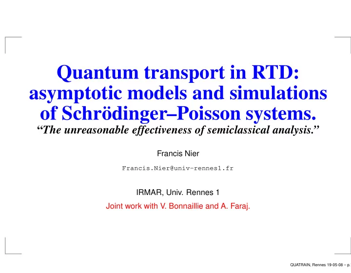
Quantum transport in RTD: asymptotic models and simulations of - PowerPoint PPT Presentation

Quantum transport in RTD: asymptotic models and simulations of Schrödinger–Poisson systems. “ The unreasonable effectiveness of semiclassical analysis.” Francis Nier Francis.Nier@univ-rennes1.fr IRMAR, Univ. Rennes 1 Joint work with V. Bonnaillie and A. Faraj. QUATRAIN, Rennes 19-05-08 – p.1

Model = k 2 Quantum wells in a (semiclassical) island ; 2 ; 3 Injection from the left (and right). Applied Bias B . i ; 2 g ( k 2 ) ; 1 λ ; 1 � B λ 1 λ 2 λ 2 λ 1 Λ λ 2 x a c 1 c 2 b QUATRAIN, Rennes 19-05-08 – p.2

Model H = − h 2 ∆ + ˜ V 0 ( x ) − W h ( x ) + V h NL ( x ) N � x − c i � � − W h ( x ) = − w i h i =1 [ H, ̺ ] = 0 F .F .E.S.S (Landauer-Büttiker) ̺ − ∆ V h NL = n � V ( a ) = V ( b ) = 0 n ( x ) ϕ ( x ) = Tr [ ̺ϕ ] h = h eff after rescaling QUATRAIN, Rennes 19-05-08 – p.2

Model Limit h → 0 → finite dimensional system: “The phenomena are governed by a finite number of resonant states” Asymptotical model Ei + − + − c c c c c i i i i+1 i+1 QUATRAIN, Rennes 19-05-08 – p.2

Model Limit h → 0 → finite dimensional system: Easy to solve numerically after some adaptations h = h eff ∼ 0 . 1 or 0 . 3 dAg Imaginary parts of resonances e − ∼ 0 OK h ≥ ≤ e − B ( h ) Comparison of tunnel effects: e − A ( h ) h h A ( h � = 0) , B ( h � = 0) , h = O (1) . Charge in a well ∼ δ c ? . Feynmann-Hellman interpolation when V h NL small. QUATRAIN, Rennes 19-05-08 – p.2

First results Bonnaillie-Nier-Patel JCP-2006 Fast numerical simulation (about 1 minute to solve 100 nonlinear problems) − > allows to study the effect of changing the values of the size of the barriers, the donnor density. . . QUATRAIN, Rennes 19-05-08 – p.3

First results Bonnaillie-Nier-Patel JCP-2006 Fast numerical simulation (about 1 minute to solve 100 nonlinear problems) − > allows to study the effect of changing the values of the size of the barriers, the donnor density. . . Provides complete bifurcation diagrams and explains the possibility of hysteresis effects. QUATRAIN, Rennes 19-05-08 – p.3

First results Bonnaillie-Nier-Patel JCP-2006 Fast numerical simulation (about 1 minute to solve 100 nonlinear problems) − > allows to study the effect of changing the values of the size of the barriers, the donnor density. . . Provides complete bifurcation diagrams and explains the possibility of hysteresis effects. At first sight, good agreement with other numerical simulations (Pinaud for Ga-As and Kumar-Laux-Fischetti for Si-SiO2). QUATRAIN, Rennes 19-05-08 – p.3

Comparison Full Schrödinger-Poisson and asymptotic model tested with the same numerical data. Check that the asymptotic model helps to guess all the possible nonlinear solutions. Check that the solutions with interaction of resonances detected with the asymptotic model make sense. Dynamics: beating effect? QUATRAIN, Rennes 19-05-08 – p.4

GaAs, 1 well, 1 resonance I-V curve Diagramm current-voltage Current BNP Current AF Current AF retour 5e+09 Current AF aller 4e+09 I (A m -2 ) 3e+09 2e+09 1e+09 0 0 0.05 0.1 0.15 0.2 0.25 0.3 B (eV) QUATRAIN, Rennes 19-05-08 – p.5

GaAs, 1 well, 1 resonance Nonlinear potential B=0.05 eV 0.025 BNP potential AF potential 0.02 0.015 potential (eV) 0.01 0.005 0 -0.005 5.5e-08 6e-08 6.5e-08 7e-08 7.5e-08 8e-08 position (m) QUATRAIN, Rennes 19-05-08 – p.5

GaAs, 1 well, 1 resonance E res − V curve Energy on the well according to the bias E 1 BNP E 1 AF 0.08 E 1 AF retour E 1 AF aller 0.06 0.04 0.02 Energy (eV) 0 -0.02 -0.04 -0.06 0 0.05 0.1 0.15 0.2 0.25 0.3 Bias (eV) QUATRAIN, Rennes 19-05-08 – p.5

Si-SiO2, 1 well, 2 resonances I-V curve Diagramm current-voltage 1.4e+12 Current BNP Current AF Current AF retour Current AF aller 1.2e+12 1e+12 8e+11 I (A m -2 ) 6e+11 4e+11 2e+11 0 0 0.5 1 1.5 2 2.5 3 B (eV) QUATRAIN, Rennes 19-05-08 – p.6

Si-SiO2, 1 well, 2 resonances Nonlinear potential B=2.04 eV 0.007 BNP potential AF potential 0.006 0.005 0.004 potential (eV) 0.003 0.002 0.001 0 -0.001 9e-09 1e-08 1.1e-08 1.2e-08 1.3e-08 1.4e-08 1.5e-08 position (m) QUATRAIN, Rennes 19-05-08 – p.6

Si-SiO2, 1 well, 2 resonances E res − V curve Energy on the well according to the bias 1 E 1 BNP E 2 BNP E 1 AF E 2 AF E 1 AF retour E 2 AF retour 0.5 E 1 AF aller E 2 AF aller 0 Energy (eV) -0.5 -1 -1.5 0 0.5 1 1.5 2 2.5 3 Bias (eV) QUATRAIN, Rennes 19-05-08 – p.6

GaAs-2 Wells-2 resonances Possible interaction of resonances c c 1 2 QUATRAIN, Rennes 19-05-08 – p.7

GaAs-2 Wells-2 resonances Asymptotic model, E res − V curve Energie dans le puits selon la diffØrence de potentiel 0.16 Energie Energie 0.15 En. crit. 0.14 0.13 0.12 Energie (eV) 0.11 0.1 0.09 0.08 0.07 0.06 0.05 0 0.02 0.04 0.06 0.08 0.1 0.12 0.14 0.16 DiffØrence de potentiel (eV) —: Energy crossing. —: The resonant energies are equal. QUATRAIN, Rennes 19-05-08 – p.7

GaAs-2 Wells-2 resonances Is it realistic ? Does it occur in the S.P . model ? QUATRAIN, Rennes 19-05-08 – p.7

GaAs-2 Wells-2 resonances Is it realistic ? Does it occur in the S.P . model ? h> 0 Crossing or E 1 = E 2 → Avoided crossings E 2 E 2 OR ? E 1 E 1 E 1 = E 2 QUATRAIN, Rennes 19-05-08 – p.7

GaAs-2 Wells-2 resonances Is it realistic ? Does it occur in the S.P . model ? h> 0 Crossing or E 1 = E 2 → Avoided crossings E 2 E 2 OR ? E 1 E 1 E 1 = E 2 Wells [5 nm, 3 . 5 nm ] Barriers [5 nm, 5 nm, 6 . 5 nm ] Previous bifurcation diagram sensitive to a a few Angström !!!. QUATRAIN, Rennes 19-05-08 – p.7

2 Wells - 2 Resonances, comparison Continuation by increasing the bias Continuation by increasing the bias 0.18 E 1 AF aller E 2 AF aller 0.16 0.14 0.12 Energy (eV) 0.1 0.08 0.06 0.04 0.02 0 0 0.02 0.04 0.06 0.08 0.1 0.12 0.14 0.16 Bias (eV) The second case is realized. QUATRAIN, Rennes 19-05-08 – p.8

2 Wells - 2 Resonances, comparison Continuation by in- and de-creasing the bias Continuation by increasing and decreasing the bias 0.18 E 1 AF retour E 2 AF retour E 1 AF aller 0.16 E 2 AF aller 0.14 0.12 Energy (eV) 0.1 0.08 0.06 0.04 0.02 0 0 0.02 0.04 0.06 0.08 0.1 0.12 0.14 0.16 Bias (eV) For some bias, both solutions coexist !! QUATRAIN, Rennes 19-05-08 – p.8

2 Wells - 2 Resonances, comparison Comparison of the bifurcation diagrams Energy on the well according to the bias 0.18 E 1 BNP E 2 BNP E 1 AF retour 0.16 E 2 AF retour E 1 AF aller E 2 AF aller 0.14 0.12 Energy (eV) 0.1 0.08 0.06 0.04 0.02 0 0 0.02 0.04 0.06 0.08 0.1 0.12 0.14 0.16 Bias (eV) Remember the strong sensitivity to the data and all the ap- proximation process. QUATRAIN, Rennes 19-05-08 – p.8

2 Wells - Beating effect At time t = 0 , the bias goes from 0 V to 0 . 08 V Current w.r.t time 2e+09 1.5e+09 Current density (Am -2 ) 1e+09 5e+08 0 0 1e-12 2e-12 3e-12 4e-12 5e-12 6e-12 time (s) Is it a (damped) beating effect ? QUATRAIN, Rennes 19-05-08 – p.9

2 Wells - Beating effect Charge densities in the first and second wells 1e+16 8e+15 6e+15 Density (m -2 ) 4e+15 2e+15 0 0 1e-12 2e-12 3e-12 4e-12 5e-12 6e-12 time (s) And T = h phys ∆ E gap up to 10%. QUATRAIN, Rennes 19-05-08 – p.9

Conclusion In spite of several “rough” approximations, the numerical results of the asymptotic model and the complete Schrödinger-Poisson model agree very well. QUATRAIN, Rennes 19-05-08 – p.10

Conclusion In spite of several “rough” approximations, the numerical results of the asymptotic model and the complete Schrödinger-Poisson model agree very well. All the semi-algebraic complexity of the bifurcation diagrams of the asymptotic model actually occurs in the Schrödinger-Poisson model. QUATRAIN, Rennes 19-05-08 – p.10

Conclusion In spite of several “rough” approximations, the numerical results of the asymptotic model and the complete Schrödinger-Poisson model agree very well. All the semi-algebraic complexity of the bifurcation diagrams of the asymptotic model actually occurs in the Schrödinger-Poisson model. The faithful and fast computations of the asymptotic model allow to design interesting test cases for the Schrödinger-Poisson problem. QUATRAIN, Rennes 19-05-08 – p.10