Quantile Estimation Definition and Examples Point Estimates Peter - - PowerPoint PPT Presentation

SLIDE 1

Quantile Estimation

Peter J. Haas CS 590M: Simulation Spring Semester 2020

1 / 20

Quantile Estimation Definition and Examples Point Estimates Confidence Intervals Further Comments Checking Normality Bootstrap Confidence Intervals

2 / 20

Quantiles

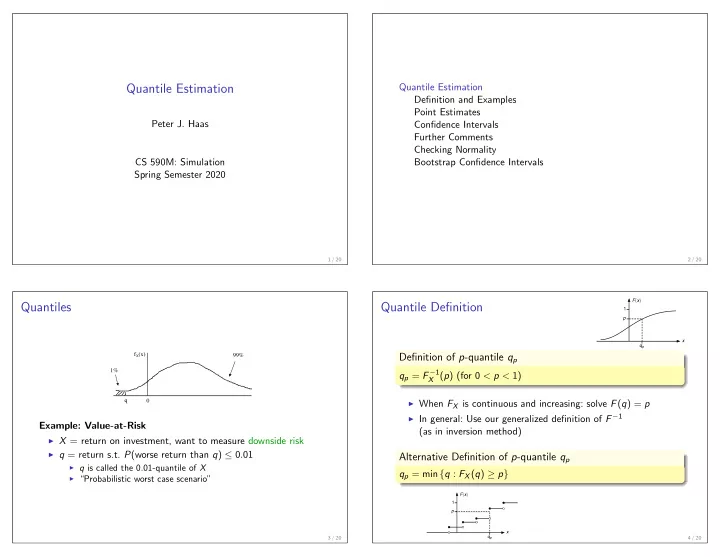
fX(x) 99% q 1%

Example: Value-at-Risk

◮ X = return on investment, want to measure downside risk ◮ q = return s.t. P(worse return than q) ≤ 0.01

◮ q is called the 0.01-quantile of X ◮ “Probabilistic worst case scenario” 3 / 20

Quantile Definition

Definition of p-quantile qp

qp = F −1

X (p) (for 0 < p < 1) ◮ When FX is continuous and increasing: solve F(q) = p ◮ In general: Use our generalized definition of F −1

(as in inversion method)

Alternative Definition of p-quantile qp

qp = min {q : FX(q) ≥ p}

4 / 20

SLIDE 2

Example: Robust Statistics

IQR

Median

◮ Median = q0.5 ◮ Alternative to means as measure of central tendency ◮ Robust to outliers

Inter-quartile range (IQR)

◮ Robust measure of dispersion ◮ IQR = q0.75 − q0.25

5 / 20

Quantile Estimation Definition and Examples Point Estimates Confidence Intervals Further Comments Checking Normality Bootstrap Confidence Intervals

6 / 20

Point Estimate of Quantile

◮ Given i.i.d. observations X1, . . . , Xn D

∼ F

◮ Natural choice is pth sample quantile:

Qn = ˆ F −1

n (p)

◮ I.e., generalized inverse of empirical cdf ˆ

Fn

◮ Q: Can you ever use the simple (non-generalized) inverse here? ◮ Equivalently, sort data as X(1) ≤ X(2) ≤ · · · ≤ X(n) and set

Qn = X(j), where j = ⌈np⌉

◮ Ex: q0.5 for {6, 8, 4, 2} = ◮ Other definitions are possible (e.g., interpolating between

values), but we will stick with the above defs

7 / 20

Quantile Estimation Definition and Examples Point Estimates Confidence Intervals Further Comments Checking Normality Bootstrap Confidence Intervals

8 / 20

SLIDE 3

Confidence Interval Attempt #1: Direct Use of CLT

CLT for Quantiles (Bahadur Representation) Suppose that X1, . . . , Xn are i.i.d. with pdf fX. Then for large n Qn

D

∼ N

• qp, σ2

n

• with

σ =

• p(1 − p)

fX(qp)

Can derive via Delta Method for stochastic root-finding

◮ Recall: to find ¯

θ such that E[g(X, ¯ θ)] = 0

◮ Point estimate θn solves 1

n

n

i=1 g(Xi, θn) = 0

◮ For large n, we have θn ≈ N(¯

θ, σ2/n), where σ2 = Var[g(X, ¯ θ)]/c2 with c = E[∂g(X, ¯ θ)/∂θ]

◮ For quantile estimation take g(X, θ) = I(X ≤ θ) − p

◮ ¯

θ = qp and θn = Qn, since E[g(X, ¯ θ)] = P(X ≤ ¯ θ) − p = 0

◮ E[∂g(X, ¯

θ)/∂θ] = ∂E[g(X, ¯ θ)]/∂θ = ∂

• FX(¯

θ)−p

• /∂θ = fX(¯

θ)

◮ Var[g(X, ¯

θ)] = E[g(X, ¯ θ)2] = E[I 2 − 2pI + p2] = E[I − 2pI + p2] = p − 2p2 + p2 = p(1 − p)

9 / 20

Confidence Interval Attempt #1: Direct Use of CLT

CLT for Quantiles (Bahadur Representation) Suppose that X1, . . . , Xn are i.i.d. with pdf fX. Then for large n Qn

D

∼ N

• qp, σ2

n

• with

σ =

• p(1 − p)

fX(qp)

◮ So if we can find an estimator sn of σ, then 100(1 − δ)% CI is

• Qn − zδsn

√n , Qn + zδsn √n

• ◮ Problem: Estimating a pdf fX is hard (e.g., need to choose

“bandwidth” for “kernel density estimator”)

◮ So we want to avoid estimation of σ

10 / 20

Confidence Interval Attempt #2: Sectioning

◮ Assume that n = mk and divide X1, . . . , Xn into m sections of

k observations each

◮ m is small (around 10–20) and k is large ◮ Let Qn(i) be estimator of qp based on data in ith section ◮ Observe that Qn(1), . . . , Qn(m) are i.i.d. ◮ By prior CLT, each Qn(i) is approx. distributed as N

• qp, σ2

k

• ◮ For i.i.d. normals, standard 100(1 − δ)% CI for mean is
• ¯

Qn − tm−1,δ vn

m , ¯

Qn + tm−1,δ vn

m

• ◮

¯ Qn = (1/m) m

i=1 Qn(i)

◮ vn =

1 m−1

m

i=1

• Qn(i) − ¯

Qn 2

◮ tm−1,δ is 1 − (δ/2) quantile of Student-t distribution

with m − 1 degrees of freedom

11 / 20

Sectioning: So What’s the Problem?

◮ Can show, as with nonlinear functions of means, that

E[Qn] ≈ qp + b n + c n2

◮ It follows that

E[Qn(i)] ≈ qp + b k + c k2 = qp + mb n + m2c n2

◮ So

E[ ¯ Qn] ≈ qp + mb n + m2c n2

◮ Bias of ¯

Qn is roughly m times larger than bias of Qn!

12 / 20

SLIDE 4

Attempt #3: Sectioning + Jackknifing

Sectioning + Jackknifing: General Algorithm for a Statistic α

• 1. Generate n = mk i.i.d. observations X1, . . . , Xn
• 2. Divide observations into m sections, each of size k
• 3. Compute point estimator αn based on all observations
• 4. For i = 1, 2, . . . , m:

4.1 Compute estimator ˜ αn(i) using all observations except those in section i 4.2 Form pseudovalue αn(i) = mαn − (m − 1)˜ αn(i)

• 5. Compute point estimator: αJ

n = 1 m m

• i=1

αn(i)

• 6. Set v J

n = 1 m−1 m

• i=1

(αn(i) − αJ

n) 2

• 7. Compute 100(1 − δ)% CI:
• αJ

n − tm−1,δ

• v J

n

m , αJ n + tm−1,δ

• v J

n

m

• 13 / 20

Application to Quantile Estimation

◮ ˜

Qn(i) = quantile estimate ignoring section i

◮ Clearly, ˜

Qn(i) has same distribution as Q(m−1)k, so

E[ ˜ Qn(i)] ≈ qp + b (m − 1)k + c (m − 1)2k2

◮ It follows that, for pseudovalue αn(i),

E[αn(i)] = E

• mQn − (m − 1) ˜

Qn(i)

• ≈ qp −

c (m − 1)mk2

◮ Averaging does not affect bias, so, since n = mk,

E[ ¯ Qn] = qp + O(1/n2)

◮ General procedure is also called the “delete-k jackknife”

14 / 20

Quantile Estimation Definition and Examples Point Estimates Confidence Intervals Further Comments Checking Normality Bootstrap Confidence Intervals

15 / 20

Further Comments

A confession

◮ There exist special-purpose methods for quantile estimation

[Sections 2.6.1 and 2.6.3 in Serfling book]

◮ We focus on sectioning + jackknife because method is general ◮ Can also use bias elimination method from prior lecture

Conditioning the data for qp when p ≈ 1

◮ Fix r > 1 and get n = rmk i.i.d. observations X1, . . . , Xn ◮ Divide data into blocks of size r ◮ Set Yj = maximum value in jth block for 1 ≤ j ≤ mk ◮ Run quantile estimation procedure on Y1, . . . , Ymk ◮ Key observation: FY (qp) = [FX(qp)]r = pr

◮ So p-quantile for X equals pr-quantile for Y ◮ Ex: if r = 50, then q0.99 for X equals q0.61 for Y

◮ Often, reduction in sample size outweighs cost of extra runs

16 / 20

SLIDE 5

Quantile Estimation Definition and Examples Point Estimates Confidence Intervals Further Comments Checking Normality Bootstrap Confidence Intervals

17 / 20

Checking Normality

Undercoverage

◮ E.g., when a “95% confidence interval” for the mean only

brackets the mean 70% of the time

◮ Due to failure of CLT at finite sample sizes ◮ Note: If data is truly normal, then no error in CI for the mean

Simple diagnostics

◮ Skewness (measures symmetry, equals 0 for normal)

◮ Definition: skewness(X) = E[(X − E(X))3]

(var X)3/2

◮ Estimator:

n−1

n

• i=1

(Xi − ¯ Xn)3

• n−1

n

• i=1

(Xi − ¯ Xn)2 3/2

◮ Kurtosis (measures fatness of tails, equals 0 for normal)

◮ Definition: kurtosis(X) = E[(X − E(X))4]

(var X)2

− 3

◮ Estimator:

n−1

n

• i=1

(Xi − ¯ Xn)4

• n−1

n

• i=1

(Xi − ¯ Xn)2 2 − 3

18 / 20

Quantile Estimation Definition and Examples Point Estimates Confidence Intervals Further Comments Checking Normality Bootstrap Confidence Intervals

19 / 20

Bootstrap Confidence Intervals

General method works for quantiles (no normality assumptions needed)

Bootstrap Confidence Intervals (Pivot Method)

• 1. Run simulation n times to get D = {X1, . . . , Xn}
• 2. Compute Qn = sample quantile based on D
• 3. Compute bootstrap sample D∗ = {X ∗

1 , . . . , X ∗ n }

• 4. Set Q∗

n = sample quantile based on D∗

• 5. Set pivot π∗ = Q∗

n − Qn

• 6. Repeat Steps 3–5 B times to create π∗

1, . . . , π∗ B

• 7. Sort pivots to obtain π∗

(1) ≤ π∗ (2) ≤ · · · ≤ π∗ (B)

• 8. Set l = ⌈(1 − δ/2)B⌉ and u = ⌈(δ/2)B⌉
• 9. Return 100(1 − δ)% CI [Qn − π∗

(l), Qn − π∗ (u)]

20 / 20