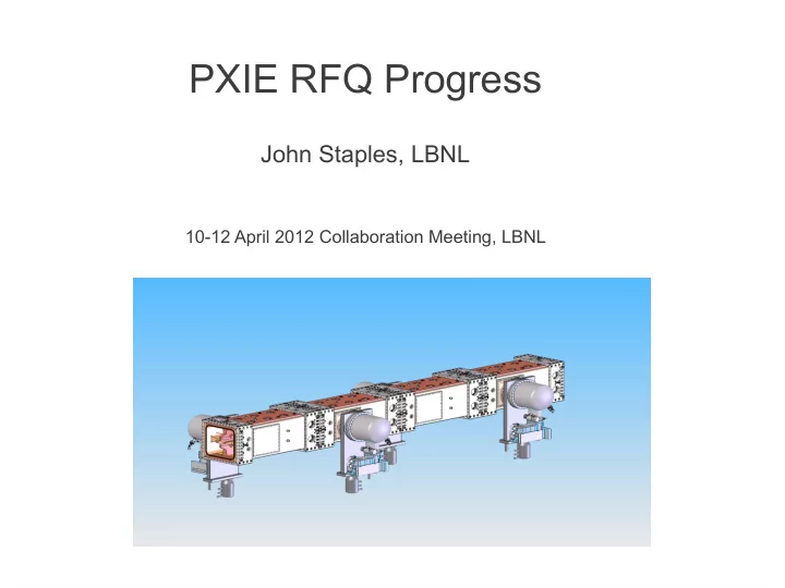
PXIE RFQ Progress John Staples, LBNL 10-12 April 2012 Collaboration - - PowerPoint PPT Presentation

PXIE RFQ Progress

John Staples, LBNL

10-12 April 2012 Collaboration Meeting, LBNL

LBNL is tasked with the design of RFQs for both FNAL (PXIE) and IMP (Lanzhou) These two CW RFQs are very similar The beam dynamics and structure design have been converging to nearly a single design, differing only in details of beam parameters. The mechanical design is compatible with available manufacturing techniques in both China and the USA. E-beam welding is used only on the ends

• f the gun-drilled water passages.

Both projects are on an accelerated schedule The beam dynamics design for PXIE and for IMP is complete

Summary

From Steve Holmes, September 2011

RFQ Parameter List

PXIE IMP Input energy 30 35 keV Output energy 2.1 2.1 MeV Frequency 162.5 162.5 MHz DC Current 5-15 5-20 mA Vane-vane voltage 60 65 kV Vane Length 444.6 416.2 cm RF Power 100 110 kW Beam Power 10.5 21 kW Duty Factor 100 100 percent Transverse emittance <0.15 mm-mrad, rms, normalized Longitudinal emittance <1.0 keV-nsec

What's New?

The beam dynamics design is frozen for both machines At FNAL's request, an exit radial matcher has been added to reduce the divergence of the output beam Transmission >99% to 10 mA Transverse emittance <0.15 pi mm-mrad to 10 mA Longitudinal emittance <0.25 pi mm-mrad (<.78 keV-deg) to 10 mA Vane length is 443.0 cm, cavity length 444.66 cm Error analysis of the structure and of the beam dynamics implications carried out LEBT chopper design integrated with the transverse acceptance of the RFQ Detailed MWS simulations of the structure (G. Romanov, FNAL) carried out

Design Highlights

Constant cross-section of structure along entire length constant transverse vane radius: only one form cutter profile needed The minimum longitudinal vanetip radius = 1.03 cm: easy design of cutter Four modules, joined with butt joints Each module assembled with brazes: no electron-beam welding, except to close the ends of the gun-bored water channels. No complex brazing operations: (No Glidcop in structure) Wall power density less than 0.7 Watts/cm2 CW (SNS was 1.7 at 6% duty factor) Pi-mode stabilizers offer very large mode separation and field stability against machining errors. 32 stabilizers used: 4 pairs/module. Mode separation, quadrupole to dipole frequency is 17.5 MHz. Length only 2.4 free-space wavelengths long (SNS was over 5 wavelengths) 80 tuners, 48 sensing loops, two drive ports

Beam Dynamics Simulations

Beam load derived from ion source emittance measurements: halo present Capture is 99.81% of 5 mA input beam Transverse output emittance 0.15 pi mm-mr Longitudinal emittance 0.68 keV-nsec Simulation using 100,000 particles, 5 mA

Input and Output phase space plots, 100,000 particles.

Input phase space derived from emittance measurement, include all ion source halo. Exit radial matcher reduces output beam maximum divergence. Beam at a waist.

Output Phase Space Distributions, x-y and phi-E, 100,000 particles

Vane Dimensions, Exit Radial Matcher

Last few cells of RFQ Exit beam nearly at a waist.

Error Analyses

Beam parameters at the end of the RFQ are modeled as a function of: Input matching conditions as a function of input Twiss parameters Input current Input centroid offset created during transition of LEBT chopper Flat gradient errors Gradient tilts Halo content for 100,000 particles Periodic field oscillation due to the 20 tuners in each quadrant All simulations use a particle distribution based on the measured emittance distribution All but the 20 tuner errors simulated with PARMTEQM; the tuner error with a modified version of PARMTEQ that allows arbitrary field variations.

2 4 6 8 10 12 14 16 0.000 0.005 0.010 0.015 0.020 0.025 0.030 0.035 0.040 0.045 0.050

x, y, z output normalized emittance vs Input Current

x-emitt y-emitt z-emitt

Input Current (mA) normalized emittance (cm-mrad, rms)

Output Emittance vs. Input Current

Optimized input current is 5 mA. Other current values use same input match. Re-matching at other currents may result in lower output emittance, so this represents the worst case away from nominal. The transverse input emittance is 0.011 pi cm-mrad, normalized, rms, derived from emittance scans of the ion source. Output longitudinal emittance at 5 mA is 0.68 keV-nsec.

• 0.5
• 0.4
• 0.3
• 0.2
• 0.1

0.0 0.1 0.2 0.3 0.4 1.0E+00 1.0E+01 1.0E+02 1.0E+03 1.0E+04

Transverse Particle Distribution

x (cm) Fraction

• 0.5
• 0.4
• 0.3
• 0.2
• 0.1

0.0 0.1 0.2 0.3 0.4 1.0E-03 1.0E-02 1.0E-01 1.0E+00 1.0E+01 1.0E+02 1.0E+03 1.0E+04

Transverse Particle Distribution

x (cm) Fraction

Transverse Particle Distribution

100,000 particles 2-gaussian fit 25% 0.5 mm rms gaussian + 75% 0.74 mm rms gaussian 2 gaussians and original spectrum fitted spectrum

2.06 2.08 2.10 2.12 2.14 2.16 2.18 2.20 2.22 1.0E+00 1.0E+01 1.0E+02 1.0E+03 1.0E+04 1.0E+05

Longitudinal Energy Distribution

KE (MeV) Fraction

2.06 2.08 2.10 2.12 2.14 2.16 2.18 2.20 2.22 1.0E-02 1.0E-01 1.0E+00 1.0E+01 1.0E+02 1.0E+03 1.0E+04 1.0E+05

Longitudinal Energy Distribution

KE (MeV) Fraction

Longitudinal Energy Distribution 100,000 particles 3-gaussian fit 71.5%, 2.5 keV rms spread + 28.0% 8.5 keV rms spread + 0.5% 20 keV rms spread The 20 keV component has a very large error bar, as it includes

• nly a few particles.

3 gaussians and the original spectrum The fitted spectrum

0.008 0.010 0.012 0.014 0.016 0.018 0.020 0.022 0.024 0.026 0.1 0.2 0.3 0.4 0.5 0.6 0.7 0.8 0.9 1

Output Longitudinal vs input Transverse Emittance

cm-mrad keV-nsec

0.008 0.010 0.012 0.014 0.016 0.018 0.020 0.022 0.024 0.026 0.000 0.005 0.010 0.015 0.020 0.025 0.030

Output vs Input transverse emittance

cm-mrad cm-mrad

Output longitudinal emittance as a function

• f transverse input

emittance. Output transverse emittance as a function

• f transverse input

emittance. 17% transverse emittance growth for input emittance

• f 0.15 mm-mrad.

Independent Parameter:

Transverse input emittance.

0.6 0.8 1.0 1.2 1.4 1.6 1.8 2.0 2.2 10 20 30 40 50 60

% Transverse emittance growth vs input Twiss alpha

Twiss Alpha Percent Transverse Emittance Growth

0.6 0.8 1.0 1.2 1.4 1.6 1.8 2.0 2.2 0.6 0.65 0.7 0.75 0.8 0.85

Longitudinal Output Emittancs vs. input Twiss alpha

Twiss Alpha Longitudinal Emittance (keV-nsec)

Output transverse and longitudinal emittance as a function of mismatch

• f Twiss parameter alpha

at RFQ entrance. Nominal value of alpha is 1.6. 5 mA input current.

Independent Parameter:

Input Twiss alpha

3 4 5 6 7 8 9 10 0.2 0.4 0.6 0.8 1 1.2

Output Longitudinal Emittance vs Twiss beta

cm keV-nsec

3 4 5 6 7 8 9 10 10 20 30 40 50 60 70

% emittance growth vs input Twiss beta

Output transverse and longitudinal emittance as a function of mismatch

• f Twiss parameter beta

at RFQ entrance. Nominal value of beta is 7 cm. 5 mA input current.

Independent Parameter:

Input Twiss beta

Scan of Output Emittance

• vs. Input Twiss Parameters

Nominal input match: Alpha = 1.6 Beta = 0.07 m (7 cm) The output emittances are minimized for the nominal value of the input Twiss

• parameters. Transmission is

greater than 99% for all cases. 5 x 5 scan of input Twiss parameters Scan beta from 0.05 to 0.09 meters Scan alpha from 1.2 to 2.0

Output Beam Parameters vs. RFQ Field Errors

Errors Considered Flat-field gradient error Field tilt error, field held constant at entrance Field tilt error, field held constant at exit Field ripple error from the tuners PARMTEQM can only simulate the first three: the field ripple is simulated with another version of parmteq with arbitrary field error.

0.88 0.90 0.92 0.94 0.96 0.98 1.00 1.02 1.04 1.06 0.6 0.7 0.8 0.9 1.0 1.1 1.2 1.3 1.4

Fractional emittance variation vs. field gradient

Fraction of nominal gradient ex, ey, ez deviation from nominal

0.88 0.90 0.92 0.94 0.96 0.98 1.00 1.02 1.04 1.06

• 0.030
• 0.025
• 0.020
• 0.015
• 0.010
• 0.005

0.000 0.005

Output Energy Deviation (MeV) vs gradient

Overall gradient fraction of nominal MeV

Output emittance and deviation from nominal 2.13 MeV output energy as a function of flat gradient error.

Independent Parameter:

Flat field gradient

• 8
• 6
• 4
• 2

2 4 6 8 0.6 0.7 0.8 0.9 1.0 1.1 1.2

Fractional emittance variation vs. field tilt

Field tilt (%), each end from center ex,ey,ez deviation from nominal

• 8
• 6
• 4
• 2

2 4 6 8

• 0.012
• 0.010
• 0.008
• 0.006
• 0.004
• 0.002

0.000 0.002 0.004 0.006

Change of output energy (MeV) vs tilt

Field tilt (%), each end from center Energy deviation in MeV

Effect on output emittance and deviation from nominal

• utput energy as a function
• f field tilt error, pivoting

around zero field error in the center of the RFQ.

Independent Parameter:

Overall field tilt

0.85 0.90 0.95 1.00 1.05 1.10 1.15 0.6 0.7 0.8 0.9 1.0 1.1 1.2 1.3

Fractional emittance variation vs. field tilt

Fraction of nominal gradient at exit; entrance field at nominal ex, ey, ez deviation from nominal

0.85 0.90 0.95 1.00 1.05 1.10 1.15

• 0.025
• 0.020
• 0.015
• 0.010
• 0.005

0.000 0.005

Output Energy Deviation vs tilt, entrance held nominal

Fraction end field of nominal MeV

Output emittance and deviation from nominal energy for zero field error at entrance, maximum at RFQ exit.

Independent Parameter:

Field tilt at exit

0.80 0.85 0.90 0.95 1.00 1.05 1.10 1.15 0.6 0.7 0.8 0.9 1.0 1.1 1.2 1.3 1.4

Fractional Emittance variation vs. Field Tilt

Fraction of nominal gradient at entrance; exit field nominal ex, ey, ez deviation from nominal

0.80 0.85 0.90 0.95 1.00 1.05 1.10 1.15

• 0.008
• 0.006
• 0.004
• 0.002

0.000 0.002 0.004 0.006 0.008 0.010 0.012

Output energy deviation vs tilt, exit end held nominal

Entrance field fraction of nominal, exit at nominal MeV

Output emittance and deviation from nominal energy for zero field error at exit, maximum at RFQ entrance.

Independent Parameter:

Field tilt at entrance

Independent Parameter:

Random Field Errors along Z 20 linacs each with 5% and 10% peak-to-peak random field error in each of 20 equal length segments along z, same distribution as number of tuners. Almost no effect on transverse emittance or capture. Plot histogram of output longitudinal emittance in MeV-deg. Zero error longitudinal emittance is 0.038 MeV-deg = 0.65 keV-nsec

0.550 0.600 0.650 0.700 0.750 0.800 0.850 0.900 0.950 1.000 1 2 3 4 5 6 7 8 9

Distribution of Longitudinal Emittance vs random field error

5% and 10% peak-peak error, 20 segments in z

Longitudinal Emittance (keV-nsec) (arbitrary)

50 100 150 200 250 300 350 400 450 500 56 58 60 62

Random Vane-Vane voltage variation

z (cm) Vane-Vane voltage (kV)

Sample random voltage variation along RFQ.

Pi-Mode Stabilizer Simulations (G. Romanov)

Quadrupole-Dipole frequency separation is 17.1 MHz.

MWS Calculation of Effect of Tuners on Field Flatness (G. Romanov)

Field Ripple due to the Tuners (G. Romanov)

Tuner sensitivity = 0.75 MHz/cm. Peak field ripple on axis less than 0.5% p-p.

0.01 0.02 0.03 0.04 0.05 0.06 0.000 0.005 0.010 0.015 0.020 0.025 0.030

Output Emittance vs peak tuner field ripple

Average all four phases of ripple

x-emitt_rms z-emitt_rms

peak ripple (fraction) emitt (cm-mrad, normalized)

Output Emittance vs. Tuner Ripple on the Field Distribution

The 20 equi-spaced tuners in each quadrant produce a variation in the field distribution. The peak-to-peak variation of the accelerating fiend is less than 1%, but is larger in the

• uter region near the tuners.

An alternate version of Parmteq was modified to include the tuner ripple on the beam

• axis. The output emittance for four phases (+sin, +cos, -sin, -cos) of the ripple

were averaged, as the absolute phase, relative to the position along the axis, will not be known until the RFQ is tuned. MWS simulation shows a p-p ripple of 0.5% at 5 mm from the axis, corresponding to a peak fraction of 0.0025

• n the plot (near zero).

The ripple in the field due to the tuners will not result in a measurable emittance increase.

Why is this design so error tolerant?

Compare parameters to SNS RFQ, which is designed for much higher current.

PXIE RFQ: a and m SNS RFQ: a and m PXIE RFQ: phis and A (Ez) SNS RFQ: phis and A (Ez)

There are no “sharp” inflection points along structure where the beam must meet criteria of proper bunch shape, space charge density, etc. The PXIE aperture is large. Most of the length of the PXIE RFQ is devoted to acceleration (plotted vs. z). Also, the PXIE RFQ has a larger aperture, thus larger transverse acceptance.

RFQ Transmission with LEBT Chopper

The 2-solenoid LEBT chopper places a parallel-plate deflector in front of the final focusing solenoid. A 0.5 cm radius aperture is placed in the entrance flange of the RFQ. The maximum chopping frequency is 1 MHz to reduce the average beam current to 1 mA. The rise/falltime of the beam due to the risetime of the electronics and the transit time of the beam through the 10-long chopper is less than 50

• nsec. During this time, the

beam will still be captured by the RFQ and sent to the MEBT.

Beam Trajectory of partially chopped beam. About 12 betatron oscillations.

What goes in of axis comes out off axis.

0.05 0.1 0.15 0.2 0.25 0.3 0.35 0.4 0.45 20 40 60 80 100 120

Transmission vs aperture radius

aperture radius (cm) transmission (%)

5 10 15 20 25 30 35 20 40 60 80 100 120

Transmission vs Deflector Field

3 different aperture radii (cm)

0.22 cm 0.25 cm 1.0 cm

Deflector field (kV/m) Transmission (%)

Transmission through the RFQ of unchopped beam as a function of an aperture at the entrance with given aperture radius The beam distribution is derived from the emittance measurement and includes halo particles. The LEBT chopper field requires at least 30 kV/m (±465 volts across a 3.1 cm gap) to extinguish the beam. A larger field will be available. Transmission through the RFQ of the chopped beam for three different aperture radii as a function of the field

• n the 11 cm long chopper.

The baseline entrance aperture radius is 0.25 cm.

RFQ Entrance Aperture

Worst-case (half-chop) particle distributions as a function of detailed RFQ gradient. There are about 12 transverse betatron oscillations along the RFQ structure. A 2% gradient increase adds about another quarter oscillation. The orbit of the partially chopped beam from the RFQ depends strongly on the actual operating gradient.

Particle and phase space distributions at the RFQ exit for various chopper fields. Almost all of the partially chopped beam stays within the unchopped beam profile 0 kV/m 5 kV/m 10 kV/m 15 kV/m

RF Structure

Structure is 444.6 cm long in four modules. 32 pi-mode stabilizers, 4 pairs in each module separate the dipole frequency to 17 MHz above the 162.5 MHz quadrupole frequency 80 tuners, 20 in each quadrant have a diameter of 6 cm, a nominal insertion

• f 2 cm, and a tuner sensitivity of 170 kHz/cm, all tuners moving together.

MWS Calculation of Cavity Frequency, Power Loss (G. Romanov)

Distribution of Power Loss on RFQ Components (G. Romanov)

Total power loss for ideal copper, no joint loss is 73.7 kW. With a 30% margin for anomalous losses, the cavity power requirement is 96 kW. Additional losses will occur in the drive loops, coaxial waveguide and circulators. Percent 40 42 1.8 2.1 7.5 6.5

Multipactoring in the RFQ Cavity

Multipactoring can occur in the cavity and in the RF drive lines. Cavity multipactoring was investigated with FISHPACT, on a 2-D slice of cavity. Fishpact was used for the APEX photoinjector cavity, which shows no MP activity. Fields were stepped over the range of operation, with emitting spots at locations around the periphery, and 6 RF start phases from 0 in steps of 60 degrees. Three FISHPACT runs with different search parameters show a minimum of activity at 60 kV vane-vane voltage. All activity is on the outer boundary of the cavity, where the electric field is low and is less likely to pull an electron

• ff the surface.

No activity is noted near the vanetips in the high E-field

• zone. The electron energy is

high so the SEY < 1.0. It is expected that no significant multipactoring will occur in the cavity.

10 20 30 40 50 60 70 80 90 1 2 3 4 5 6 7

Multipactoring Probability vs. Vane-Vane Voltage

Voltage (kV) (arbitrary)

RF Driveline Multipactoring

The APEX photoinjector runs 100 kW CW at 187 MHz (1.3 GHz / 7) and has two loop couplers, each delivering 50 kW. The RF windows are located 90 cm away from the drive loops. Severe multipactoring in the vacuum sections

• f the drive lines was observed.

The multipactoring was suppressed by surrounding them with 100 gauss solenoid coils. We may shorten the drive lines and move the windows much closer to the coupling loops to eliminate possible magnetic fields at the photocathode. A similar situation may affect the PXIE RFQ drive lines and should be taken into account. RF Windows

Tuning the RFQ

The RFQ will be tuned with a bead-pull of a substructure and of the entire structure, and the 48 sensing probes, 3 / quadrant / module will be calibrated. We will pull only one bead in one quadrant as the pi-mode stabilizers strongly lock the fields in the four quadrants together. (Picture is of SNS 1-module cold model.)

Perturbations to Field Flatness: Tuning

Entrance 6-cell radial matcher Frequency perturbation of +0.33 MHz causes an uncorrected field tilt of +45% at the exit. Corrected by modifying the entrance end cutbacks in the vanes Effect of the modulations of the vane tips Local frequency variation -0.2 to +0.5 MHz,

• r an overall perturbation of +0.17 MHz,

causing a field tilt of -18% at the exit. Corrected by the local tuners. Group tuner sensitivity: +0.46 MHz/cm. Initial tuner insertion is 2 cm, or +0.92 MHz. Pi-Mode Stabilizers: -4.5 MHz frequency shift “Bare” (Superfish) frequency about 3 MHz high before tuners, stabilizers and ends added.

Field Perturbation from Cold to Hot

The waterflow circuits in each of the four modules will be in the following directions: The change is water temperature in each module produces a frequency shift of 10 kHz from

• ne end to the other (blue). This results in a variation of the field of 0.025% peak-peak(red).

This field variation will not be present during low-level tuning and will not be significant for full-power operation.

Lessons Learned from other RFQs

Most run just fine, but there have been problems with some. SNS: Two instances of frequency jumps with field redistribution. Required

• retuning. Pi-mode stabilizers probably kept the fields close to nominal even though

a quadrant asymmetry may still exist. Investigated thoroughly, cause not found. RFQ continues to operate satisfactorily. Other RFQs: Sloppy assembly Inability to gain access to structure through surrounding jacket Insufficient thermal capability at required gradients Poor mechanical design Four-rod warping problem Poisoning from severe vacuum accident Discharges due to poor vacuum at entrance PXIE RFQ: None of the above problems are expected for the PXIE RFQ. The thermal wall loading is 1/3 of SNS, the peak gradient is 1.2 kilpatrick. Possible multipactoring problems with the drive loops has been recognized. The water passages are gun-bored into the structure itself: no exoskeleton. Vacuum at the RFQ entrance will be in the low 7's due to a small entrance aperture and a 1.5 meter distance from the ion source. Beam loss in the RFQ, including chopping, is expected to be very small.

Recap: Issues Addressed

Design frozen: final engineering proceeds Easily meets requirements High acceptance, 0-10 mA characteristics, low output divergence Error Analysis Current dependence Beam quality dependence on field errors Large field errors results in small emittance growth RF Design Stabilizers, mode separation, tuning Large separation of quadrupole and dipole modes Large immunity to asymmetry and machining errors RF Power issues Power distribution within structure No expected multipactoring in cavity, but watch drive lines. Lessons learned from other RFQs Design avoids issues that have arisen in other RFQs