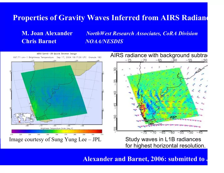
SLIDE 1 Properties of Gravity Waves Inferred from AIRS Radianc
- M. Joan Alexander NorthWest Research Associates, CoRA Division
Chris Barnet NOAA/NESDIS
Alexander and Barnet, 2006: submitted to JAS
Image courtesy of Sung Yung Lee – JPL Study waves in L1B radiances for highest horizontal resolution. AIRS radiance with background subtrac
SLIDE 2
- Ice cloud formation with subsequent effects on:
- Stratospheric dehydration
in the tropics
- Polar ozone loss
- Cirrus radiative effects
Global Effects of Gravity Waves
- Driving the observed zonal mean
circulation:
- QBO in stratosphere winds
- Drag force on the winter jet
- Timing of summer easterlies
This process currently parameterized in most global models. Observational constraints needed.
SLIDE 3
UARS-MLS Gravity Wav Temperature Variance
Long-Vertical Scale |T'| (Wu and Waters, 1996) max |T'| ~ 0.2K
GPS Gravity Wave Potential Energy
Short-Vertical Scale |T'|2 (Tsuda et al., JGR, 2000) max |T'| ~ 2K
SLIDE 4 Effective Weighting Functions for gravity wave observations
(schematic)
Sub-limb Viewing Limb Viewing Nadir Viewing
SLIDE 5
- Probability of Observation ~ 1 / Cgz
FAST = Large Cgz ~ ω / m ~ Ch k / m FAST ~ high frequency, long vertical scale, short horizontal scale, high phase speed. Fast waves are harder to observe.
- There is therefore a tendency to overemphasize the slow waves
in long-term averaged data. Momentum Flux ~ (k/m) x Temperature Variance
- Fast waves will supply a disproportionate share of the global
gravity wave momentum flux.
SLIDE 6
15 micron band 4.2 micron band
In collaboration with Chris Barnet, we are examining AIRS radiances in two CO2 emission bands in the stratosphere Kernel Functions
SLIDE 7
Focus on the 667.77 cm-1 AIRS Channel in the 15 micron band
The depth of the weighting functions and the near-nadir view angles of AIRS mean there will be little or no response to waves with vertic wavelengths less tha 12 km.
AIRS => Focus on long vertical scale, short horizontal scale waves = Fast Waves! => Show horizontal propagation direction and resolve the short horizontal scale waves undersampled in previous measurements.
SLIDE 8 Wave Identification Analysis:
- For each cross-track row (x) of AIRS data:
- Interpolate to constant resolution = 18.9km.
- Compute the S-Transform of each row.
- Compute the cospectrum between
adjacent rows => (amplitude, phase).
- Compute the average cross-track covariance
spectrum of the AIRS Granule.
- Find the peaks in this average spectrum.
- Store amplitude(x,y) phase(x,y) for these
dominant scales.
- Use the phase shift between rows to compute
the amplitude-weighted y-wavelength (x,y).
- We perform a wavelet analysis in the cross-
track x-direction using the S-transform wavelet (Stockwell et al., 1996)
x
SLIDE 9
S-Transform Results (raw) Sep 10, 2003 Granule 4
SLIDE 10
Sep 10, 2003 Granule 4
WAVE ANALYSIS STATISTICS
SLIDE 11
Mountain Wave Study Select All Granules intersecting -56<lat<-36, -76<lon<-56 Month of September 2003
40 AIR Granule location
+ High point a
each latitude Ridge definitio for this study.
SLIDE 12
All Granules (-56<lat<-36, -76<lon<-56): September 1-30, 2003
(40 Granules = 486,000 data points)
SLIDE 13
have short wavelengths, ~ 100km.
wavelengths is observed ranging up to 500 km.
Distribution of wave amplitudes and their horizontal wavelengths:
(Total of 40 granules)
NUMBER OF PIXELS
All Granules (-56<lat<-36, -76<lon<-56): September 1-30, 2003
SLIDE 14
angle would be 180o.
at an angle of 185o for weak events. The “weak events” that
likely stronger events with short wavelengths that are highly attenuated.
fewer in number, but also peak near 180o.
Distribution of wave amplitudes and their propagation direction relative to the background wind: (Total of 40 granules) All Granules (-56<lat<-36, -76<lon<-56): September 1-30, 2003
NUMBER OF PIXELS
SLIDE 15 Background Wind Effects on Visibility of the Waves Example: Sep 1, 2003 Granule 196
Waves appear
winds and propagate in the direction ~190 degrees upstream of the wind direction.
SLIDE 16 (from Alexander and Holton [
SLIDE 17 NOISE=.72
Average amplitude shows an increasing trend where background winds exceed ~ 40 m/s.
Data from all granules show wave amplitudes increase dramatically
wherever background winds exceed 40 m/s. For a given background wind speed, the average wave amplitudes are also largest when the waves propagate perpendicular to the background wind.
SLIDE 18
Data from all granules show wave amplitudes increase dramatically
wherever background winds exceed 40 m/s.
40 m/s is a magic number for seeing mountain waves in AIRS data: * Minimum vertical wavelength λz = 12km * Mountain wave frequency ω0 = 0 phase speed c0 = 0 intrinsic frequency ω = ω0 − Uk = -Uk intrinsic phase speed c = c0 – U = -U * Gravity wave dispersion relation (simplified form): | λz | = 2π|U|/N * N ~ .02 s-1 (roughly constant), so for U = 40 m/s => λz = 12.5 km
SLIDE 19 Case Study: Sep 10, 2003 Granule 44
Radiance perturbations: color Stratospheric wind vectors: pink Surface wind vectors: blue
Wind divergence at 40 km (left) and 5 km (right)
ECMWF shows similar wave in both wind and temperature fields: (collaboration with H. Teitelbaum)
Source traced to a surface front east
Penninsula
SLIDE 20 Case Study: Jan 12, 2003 Granule 167
Waves generated by tropical convection
seen in AIRS radiances Ongoing work Model studies waves generate by Darwin-are convection.
SLIDE 21 Conclusions
- Image data like AIRS offer opportunities to study wave events
- Give amplitudes, wavelengths,
and propagation directions at high horizontal resolution.
compared to detailed wave source models and used to improve those models and constrain parameterizations.
- Current data are limited to only long vertical wavelength waves,
which also have high horizontal phase speeds, fast propagation speeds and a high degree of intermittency.
- Such waves are underestimated in global averaged data but may
carry a large fraction of the net gravity wave momentum flux.
PDF of Patagonian mountain waves