Prognostic/Diagnostic Health Management System (PHM) for Fab - - PDF document

Prognostic/Diagnostic Health Management System (PHM) for Fab Efficiency Chin Sun Quality Wise Knowledge Solutions San Jose, CA USA email csun@qwiksinc.com Kevin Nguyen Global CyberSoft. Santa Clara, CA USA email Kevin@globalcybersoft.com Long Vu Global CyberSoft. Round Rock, TX USA email Longvu@globalcybersoft.com Scott G. Bisland Sematech / ATDF Inc. Austin, TX USA email scott.bisland@atdf.com Abstract In this work, a Prognostic/Diagnostic approach was made to use knowledge-based system to accelerate the proc- ess/equipment faults detection and classification. The do- main knowledge within the Fab environment can be either captured by PHM systems or populated by the experienced

• engineers. With the implementation of the proposed PHM

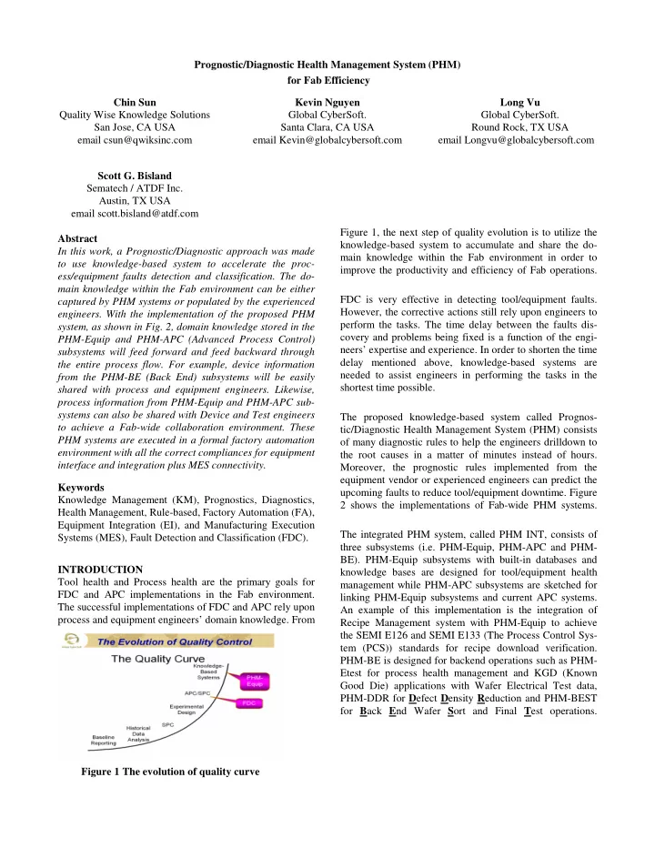
system, as shown in Fig. 2, domain knowledge stored in the PHM-Equip and PHM-APC (Advanced Process Control) subsystems will feed forward and feed backward through the entire process flow. For example, device information from the PHM-BE (Back End) subsystems will be easily shared with process and equipment engineers. Likewise, process information from PHM-Equip and PHM-APC sub- systems can also be shared with Device and Test engineers to achieve a Fab-wide collaboration environment. These PHM systems are executed in a formal factory automation environment with all the correct compliances for equipment interface and integration plus MES connectivity. Keywords Knowledge Management (KM), Prognostics, Diagnostics, Health Management, Rule-based, Factory Automation (FA), Equipment Integration (EI), and Manufacturing Execution Systems (MES), Fault Detection and Classification (FDC). INTRODUCTION Tool health and Process health are the primary goals for FDC and APC implementations in the Fab environment. The successful implementations of FDC and APC rely upon process and equipment engineers’ domain knowledge. From Figure 1, the next step of quality evolution is to utilize the knowledge-based system to accumulate and share the do- main knowledge within the Fab environment in order to improve the productivity and efficiency of Fab operations. FDC is very effective in detecting tool/equipment faults. However, the corrective actions still rely upon engineers to perform the tasks. The time delay between the faults dis- covery and problems being fixed is a function of the engi- neers’ expertise and experience. In order to shorten the time delay mentioned above, knowledge-based systems are needed to assist engineers in performing the tasks in the shortest time possible. The proposed knowledge-based system called Prognos- tic/Diagnostic Health Management System (PHM) consists

• f many diagnostic rules to help the engineers drilldown to

the root causes in a matter of minutes instead of hours. Moreover, the prognostic rules implemented from the equipment vendor or experienced engineers can predict the upcoming faults to reduce tool/equipment downtime. Figure 2 shows the implementations of Fab-wide PHM systems. The integrated PHM system, called PHM INT, consists of three subsystems (i.e. PHM-Equip, PHM-APC and PHM- BE). PHM-Equip subsystems with built-in databases and knowledge bases are designed for tool/equipment health management while PHM-APC subsystems are sketched for linking PHM-Equip subsystems and current APC systems. An example of this implementation is the integration of Recipe Management system with PHM-Equip to achieve the SEMI E126 and SEMI E133 (The Process Control Sys- tem (PCS)) standards for recipe download verification. PHM-BE is designed for backend operations such as PHM- Etest for process health management and KGD (Known Good Die) applications with Wafer Electrical Test data, PHM-DDR for Defect Density Reduction and PHM-BEST for Back End Wafer Sort and Final Test operations. Figure 1 The evolution of quality curve

An example of failing oxygen sensor prognostic rule implementation to demonstrate the effectiveness of the PHM system is given in Figure 7 and 8. This approach will be described in detail in this presentation. The user-friendly rules development and test environment will also be dem-

• nstrated.

With the implementation of the proposed PHM system as shown in Fig. 2, domain knowledge stored in the PHM- Equip and PHM-APC subsystems will feed forward and feed backward through the entire process flow. For example, device information from the PHM-BE subsystems will be easily shared with process and equipment engineers. Like- wise, process information from PHM-Equip and PHM-APC subsystems can also be shared with Device and Test engi- neers to achieve a Fab-wide collaboration environment. Figure 2: Components of a Fab-wide PHM Systems EXPERIMENTAL The datasets from TI’s (Texas Instruments) experiment were utilized to illustrate PHM’s capabilities in faults detec- tion and classification. The training and test datasets from the 129 wafers can be downloaded from this URL: http://software.eigenvector.com/Data/Etch/index.html. There are 21 variables from a LAM 9600 Metal Etcher and 129 OES (Optical Emission Spectroscopy, 245 to 800 nm) parameters from the OES fiber optics sensors as shown in Table 1. The training dataset consists of 108 wafers taken during 3 experiments. There were 21 wafers with intention- ally induced faults as shown in Table 1. The experiments were run several weeks apart and data from different ex- periments has a different mean and somewhat different co- variance structure. Therefore, these three datasets were ana- lyzed separately to avoid system degradation effects. METHODS A Health Examination system is a multidimensional system. In Most of the multidimensional systems, the objective is to make a decision based on several input characteristics (“characteristics” are also referred to as “variables”). Tradi- tionally, Mahalanobis distance (MD) is used to determine the similarity of a set of values from an unknown sample to a set of values measured from a collection of known sam-

• ples. The original MD calculations can be obtained from

Mahalanobis (1936). In the present method, MD is suitably scaled and used to construct a scale to monitor the condi- tion of entities of a multidimensional system. The method has a new way of deciding which variables are useful (im- portant) using Orthogonal Arrays (OA’s) and S/N ratios. A discussion on OA’s and S/N ratios is given in Taguchi (1987). Unlike in other methods, in this method the abnor- malities (“abnormalities” are also referred to as “abnor- mals”) do not constitute a separate population – they are

• unique. Therefore, our problem is not one of classification

into two populations of normal and abnormal. The meas- ures and methods used in Mahalanobis-Taguchi-System (MTS) are data analytic (using the measures of descriptive statistics and principles of Taguchi Methods) rather than usual probability based inference. THE MAHALANOBIS-TAGUCHI SYSTEM (MTS) Figure 3. Multidimensional diagnosis system Table 1: Variables and faults listing

A typical multidimensional system used in MTS is shown in Figure 3. In this figure X1, X2,…,Xn correspond to the variables which provide a set of information to make a de-

• cision. Using theses variables, MS (Mahalanobis Space) is

constructed for the healthy group, which becomes the refer- ence point for the measurement scale. After constructing the MS, the measurement scale is justified by considering the known abnormals. The abnormals have to be checked with the given input signals and in the presence of the noise fac- tor (if any). MTS is a diagnostic and forecasting tool for identifying the degree of abnormality of observations based on multivariate variables of “normal” group of observations. Examples of normal groups are the healthy persons in a drug diagnostic, the persons with good credit in a credit evaluation, and the good products in a product inspection process. To apply MTS, the first step is to define and sample “normal” obser- vations to construct a reference space, which is also re- ferred to Mahalanobis Space (MS), and then we identify whether the created Mahalanobis Distance (MD) has the ability to differentiate “normal” group from “abnormal” group.

• Phase 1: Construct a measurement scale with MS as

the reference In order to construct a measurement scale, we need to col- lect a set of “normal” observations and standardize the vari- ables of these observations to calculate the Mahalanobis distances (MDs). MD measures distances in multidimen- sional spaces by taking into account the correlation among

• variables. In classical methods, Mahalanobis Distance is

used to find the “nearness” of an unknown point from the mean of a group. In MTS, the MD in (1) is the original MD divided by k. The MDs define a Mahalanobis Space (MS), which provides a reference point for the measurement scale. The following is the formula used to calculate MDs: Where Si= standard deviations of i – th variable, C-1 = the inverse of correlation matrix, k = number of variables, n = number of observations, T = transpose of the standard vec- tor. According to Dr. Taguchi [4] the average value of MD is equal to 1 for all the observations in MS, which is why MS is also called unit space. Phase 2: Validate the measurement scale For validating the measurement scale, we choose

• bservations outside of MS, usually “abnormal” observa-
• tions. In the MTS, the decision maker chooses solely the

variables that are required for creating an MTS measure- ment scale, so these variables need to be examined again to make sure they are properly selected. After the measure- ment scale is established, we need to use observations out- side of MS to evaluate if these variables are suitable. If the numbers of abnormal observations are t, we use the average and standard deviation and correlation matrix of these “normal” observations to calculate the MD in the “abnor- mal” observations. According to the MTS theory, the MD

• f “abnormal” observations will be larger than the MD of

“normal” observations, if this is a good scale. RESULTS - Faults Detection Step 1: Define the problem In the MTS approach, we need to define “normal”

• bservations to construct the MS. In this example we define

three groups of training datasets as “normal” observations as shown in row 2 of Table 2, and use the MS constructed from these “normal” observations to differentiate the other three test datasets as shown in row 3 of Table 2. Table 2 Experiment Split Information Experiment No. Experiment 1 Experiment 2 Experiment 3 Training Dataset Wafers 1 - 34 Wafers 35 - 71 Wafers 72 - 108 Test Dataset Wafers 1 – 9 Wafers 10 - 15 Wafers 16 - 21 Step 2: Define response/control variables We define the 21 machine state variables and 129 OES variables as the control factors, and MD as the response variable.

Step 3: Construct the “Full Model MTS Measurement Scale” In this step, we collect “normal” observations to construct the “Full Model MTS Measurement Scale”. Table 3, 4 and 5 show the three different experiment results. The measurement scale is constructed by training datasets while the capability of measurement scale is demonstrated by test datasets. Table 3 shows the MDs distribution be- tween this “normal” data and the other “abnormal” data. The average of the MDs for normal data of Experiment 1 is 0.999713, which is very close to 1. This is very close to the theory of the MTS. The range of the MDs for abnormal data for Experiment 1 is 2.75 – 43.815. The results of ex- periment 2 and 3 are shown in Table 4 and 5, respectively. Table 3 Experiment 1 Machine State Variables results Datasets Experiment 1 Training datasets MD Threshold limit, average MD 1.83727 (0.999713) Test datasets MDs (2.75 – 43.815) Table 4 Experiment 2 Machine State Variables results Datasets Experiment 2 Training datasets MD Threshold limit, average MD 1.894087 (0.999725) Test datasets MDs (2.4498 – 201.701) Table 5 Experiment 3 Machine State Variables results Datasets Experiment 3 Training datasets MD Threshold limit, average MD 1.989112 (0.999718) Test datasets MDs (2.453 – 5.758) Step 4: Validate the ability of the measurement scale According to the MTS theory, the MD of “abnormal” ob- servation will be larger than the MD of “normal” observa- tion, if this is a good measurement scale. In this study, we use a test sample to validate and calculate the MD for each

• bservation. The MD threshold limit is computed from the

training dataset with %95 confidence level. The result shows that the measurement scale constructed by all 21 machine state variables is good, since all the test wafers’ MD are all greater than the respective threshold limit. Therefore, they were all identified as faulty wafers. Figure 4 Signal Plots vs time for Machine State Variables RESULTS - Faults Classification For machine state faults detection, a model with 21 vari- ables (i.e. 21 dimensional system) was built to detect sys- tem faults. The 21x21 correlation matrix contains all the correlated information among the 21 variables. Similar to the machine state model, a 129x129 model with 129 vari- ables was also built using OES dataset. In order to find out the variables associated with the system faults, we need to be able to distinguish the signal pattern shift of each variable as shown in Figure 4 between the test dataset and the model built from the training dataset. There- fore, we need to build pattern recognition models for each

• variable. For each variable in the training dataset, we plot

the signal pattern vs time. Then we converted the image

into a digital data table. The columns of this data table were carefully chosen to maximize the pattern recognition capa- bilities using MTS methodology. The results of fault classi- fication using MTS pattern recognition are shown in Table

• 6. Note that in Table 6, test wafer 2 and test wafer 18 have

the same four machine state variables associated with the RF-12 system fault. This result confirms that our MTS pat- tern recognition technology was able to capture the vari- ables associated with the system faults. Table 6 Machine State Variables associated with Ma- chine State Faults The variables associated with the system faults will then be converted to either prognostics or diagnostics rules by the system’s built-in Pattern Signature capture program as shown in Figure 5. Figure 5. Create Diagnostic Rule from pattern signature Prognostics/Diagnostics rules can be either generated auto- matically from pattern signature capture or can be popu- lated by experienced personnel. With 20 fault diagnos- tic/classification rules in the system, PHM system’s Faults detection and classification summary is shown in Figure 6. Note that from Figure 6, FDC status (i.e. fault or normal), System Health Index and parameters associated with faults allows the equipment engineers to generate pareto analysis and other statistical summaries to keep track of equipment performance and utilization. Figure 6. PHM Fault Detection and Classification Summary Example of Prognostic Rule for oxygen sensor Figure 7 shows the pattern signature for a failing oxygen sensor compared to a normal oxygen sensor shown in Fig- ure 8. It will be beneficial to report the failing sensors with limited life time left to the equipment engineers for proac- tive system maintenance. Figure 7 Failing oxygen sensor Figure 8. Normal oxygen sensor With PHM’s built-in signal pattern recognition technology, the failing oxygen sensor’s %img_off_target (i.e. image off target value) is 22.87% compared to the normal oxygen sensor signal of near 0%. With the appropriate setup of rules as shown in Figure 9, it is very easy to detect the symptoms and report them to the equipment engineers for appropriate corrective actions.

Figure 9. Failing oxygen sensor prognostic rule

CONCLUSION The domain knowledge stored in the PHM-Equip and PHM-APC subsystems (Figure 2) will feed forward and feed backward through the entire process flow. Wafer Elec- trical Test information from the PHM-Etest subsystem will be easily shared with process and equipment engineers. Likewise, process and equipment operational information from PHM-Equip and PHM-APC subsystems can also be shared with Device and Test engineers to achieve a Fab- wide collaboration environment. As a result, equipment and processes are monitored “real time” allowing for immediate notification, identification and suggested remediation of both equipment and process issues. This in turn provides decreased scrap wafers, improved process, quality control, and increased yield to the Fab environment. Additionally, with a Knowledge Base of countless years of equipment maintenance knowledge, equipment repairs, spares and warranty issues can be tracked in a single location. Even small gains in yield can provide millions of dollars in in- creased revenues to any Fab. ACKNOWLEDGMENTS The authors would like to thank Sematech /ATDF Inc for supporting this study. REFERENCES [1] The Emerging Role For Data Mining. -- SOLID STATE TECHNOLOGY 11/99 Magazine Volume 42 Issue 11 [2] Hand, D. J., Constructed and Assessment of Classifica- tion Rules, John Wiley and Sons, Chichester (1997). [3] Johnson, R. A. and Wichern, D. W., Applied Multi- variate Statistical Analysis, McGraw-Hill Press, New York (1998). [4] Taguchi, G., S. Chowdury, and Wu, Y., The Maha- lanobis-Taguchi System, McGraw-Hill Press, New York (2001). [5] Taguchi, G., R. Jugulum, S. Taguchi, and Wilkins, J.O., “Discussion - A review and analysis of the Mahalano- bis-Taguchi system,” Technometrics, February 45, 16- 21 (2003). [6] Taguchi, G. and R. Jugulum, “New Trends in Multi- variate Diagnosis,” Sankhy: The Indian Journal of statistics, 62, Series B, 2, 233-248 (2000). [7] Taguchi, G. and R. Jugulum, The Mahalanobis- Taguchi Strategy, John Wiley and Sons Press, New York (2002). [8] Woodall, W. H., R. Koudelik, K. L. Tsui, S. B. Kim, Z.

• G. Stoumbos, and C. P. Carvounis, “A review and

analysis of the Mahalanobis-Taguchi system,” Tech- nometrics, February, 45, 1-15 (2003).. BIOGRAPHY Chin Sun received the B.S. degree in Chemistry from Na- tional Chung-Hsing University in Taiwan, R.O.C. in 1980 and the M.S. degree in electrical engineering from the Uni- versity of Arizona in 1988. For the last 17 years, Mr. Sun worked for IDT and AMD as a yield enhancement engineer.

• Mr. Sun holds 4 US Patents. He is currently the President

and CTO of Quality Wise Knowledge Solutions.

Kevin Nguyen offers 25 years of extensive entrepreneurial ex- perience in system integration and internet-related activities, spe- cializing in semiconductor IC design and manufacturing layout. He founded several factory automation consulting companies in Silicon Valley. Prior to being an entrepreneur, Kevin worked as senior technical professional for various major US hi-tech compa- nies including IBM, Honeywell, and Boeing Computer Services. Kevin earned a BSIE from University of Illinois and a MSIE from University

• f

Cincinnati. Long Vu has over fifteen years experience in developing ad- vanced analytical equipment for the Semiconductor Manufactur- ing Industry, most recently in X-ray metrology, and hold patents

• n x-ray technologies that have gained worldwide market accep-
• tance. Long received the B.S. Electronics Engineering degree

from New Jersey Institute of Technolo-gies (NJIT) in 1994. Scott Bisland is the Equipment Services Manager at Se-matech / ATDF Inc., Advanced Technology Development Facility, Austin

• Texas. Seasoned Project Manager of successful multi-million

dollar conversion and installation projects. Scott received the B.S. Electronics Engineering degree from Texas A & M University, College Station Texas in 1987. In 1989, Scott was an instructor of Laser Electro-Optics at Texas State Technical College, Waco Texas.