Problems A problem (in Computer Science) specifies an input/output - - PDF document

1/23/2010 1 A Constant-Space Model of Computation for First-Order Queries

Steven Lindell Haverford College USA

1

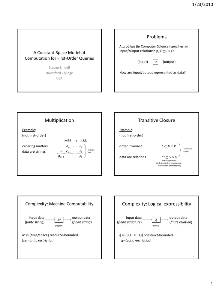
Problems

A problem (in Computer Science) specifies an input/output relationship, P  I  O. (input) (output) How are input/output represented as data? P

2

Multiplication

Example: (not first-order) MSB  LSB

• rdering matters

data are strings

• rdered

bits

dn-1 · · · d0  en-1 · · · e0 p2n-1 · · · · · · p0

3

Transitive Closure

Example: (not first-order)

• rder invariant

E  V  V data are relations E+  V  V

unordered graphs matrix operation (independent of simultaneous row/column permutations)

4

Complexity: Machine Computability

M is {time/space} resource-bounded. [semantic restriction] input data (finite string) M

• utput data

(finite string)

program

5

Complexity: Logical expressibility

 is {SO, FP, FO} construct-bounded [syntactic restriction] input data (finite structure) 

• utput data

(finite relation)

formula

6

1/23/2010 2

Logical Definability

second-order = polynomial-hierarchy fixed-point(<) = polynomial-time = P first-order(+, *) = constant (parallel) time  L = constant (serial) space

7

Logical Framework

Finite relational structure: A, R1, …, Rk, Q First-order queries: x, y, z, … individual variables (over A) =, Ri atomics , ,  boolean connectives x, x quantification (over A)

finite domain query (defines a new relation) relations

8

Example: Graph Simplicity

directed graph: G = V, E (binary relation) E  V  V Simplicity:

• (x  V)[E(x, x)] 

no self-loops (y)(z)[E(y, z)  E(z, y) undirected edges

9

Example: Linear Ordering

total linear order:

• (x < x)

irreflexive (x  y)  [(x < y)  (y < x)] total [(x < y)  (y < z)]  (x < z) transitive

10

Binary String Structures

{0, 1, …, n  1}, <, U

Example: w = 1010 is represented by {0, 1, 2, 3}, <, {0, 2}, with 0 < 1 < 2 < 3.

< < < 1 2 3

set of positions orders the positions indicates the locations of 0’s and 1’s

11

Arithmetic & bit

Definition: For w  {0, 1}*, |w|, <, bit, {i: wi = 1} where bit(i, j)  the jth bit of i is 1 (numerical predicate) 0 < 1 < … < (n  1) n, +,  0  a, b, c < n a + b = c a  b = c

12

1/23/2010 3

Examples

n is even?  FO(+) \ FO(<) n is prime?  FO(+, ) \ FO(+) a ^ b = c  FO(+, ) FO(<, bit) = FO(+, ) PARITY  FO(any numerical predicates, U) [FSS] (asks if |U| is even)

13

Logspace Computation

Off-line Turing machine (sub-linear space):

size = n read-only input tape read/write work tape finite control heads space = O(log n) space = O(1)

14

Bidirectional multi-head DFA

Each head can be thought of as an integer “cursor” holding log n bits of storage, so this model is equivalent to logspace.

read-only input tape finite state control

. . .

15

Circuit model (non-uniform): AC0

inputs w/ negations

Constant (parallel) time

… n inputs . . . … … constant depth polynomial size

16

PRAM model (uniform)

resolve conflicts in various ways FO(+, ) = PRAM(O(1) time) [Immerman]

global read/write memory

. . .

O(nO(1)) processors

17

Regular Languages

On word models REG = mSO(<) star-free REG = FO(<)

18

1/23/2010 4

Inclusions

ALOGTIME (uniform NC1) REG FO(<,bit) FO(<,mod)

PARITY = {w: even # of 1’s}  REG\FO(<,bit) EQUAL= {w: equal # of 0’s and 1’s}  ALOGTIME\... EVEN = {w: |w|# is even}  FO(<,mod) MIDDLE = {0n1n: n = 0, 1, …}  FO(<,bit) \REG

19

Finite-State Machines

FSM: single oblivious head flip/flops & gates

read-only input tape finite-state control

single scan

Chart finite automata proposed model I/O access single scan multiple passes control state machine restricted mechanism

20

Proposed Model

multiple oblivious heads destructive read

read-only input tape finite control

. . .

1 flip-flop (one bit) single token of information: cannot be split or shared (a quantum bit)?

21

Constant-Space Machine (hardware)

• multiple heads / multiple passes
• flow of information
• actual read/write storage
• uniform version of formula width (constant-width circuit

with fan-out one) read-only input tape positional control

. . .

comparators binary counters boolean calculation relative, absolute

fixed no. of heads

read-once variables

• blivious program

movement data

head position

22

Constant-Space Program (software)

b boolean variable I[h] input bit under head h i < j head i is left of head j bit(i,j) jth bit of head i’s counter AND, OR, NOT to form expressions b := e boolean assignment P; Q; sequential composition LOOP h sequential iteration P; (head h scans whole tape) IF e THEN P; conditional (not allowed)

• Program syntax guarantees: obliviousness; read-once
• Finiteness implies: constant-space; polynomial-length

23

Sample Program: Parity

Compute the parity of a = a1 … an: p := 0; {initialize} LOOP h {LSB to MSB} p := a(h) XOR p; {exclusive-or} Note: p violates the read-once condition in .

24

1/23/2010 5

Sample Program: Binary addition

Binary addition: an … a1 + bn … b1 = c sn … s1 c := 0; {initialize carry} LOOP h {from LSB to MSB} s(h) := a(h) XOR b(h) XOR c c := a(h) AND b(h) OR c AND ((a(h) OR b(h))

• c in output statement doesn’t count since s is write-only
• c occurs once in re-parenthesized majority function

25

Main Result

Theorem: A (binary) language L  {0, 1}* is recognizable by a read-once constant-space program if and

• nly if it is definable by a first-order formula

with arithmetic

26

Time / Space Duality

Corollary (Duality principle): A problem is computable by a read-once constant-space serial algorithm if and only if it is computable by a constant-time parallel algorithm [extends previously known duality to below O(log n)].

28

Carry look-ahead (binary addition)

𝑡 𝑗 = 𝑏 𝑗 ⊕ 𝑐 𝑗 ⊕ 𝑑 𝑗 where 𝑑 𝑗 = ∃𝑘 [𝑘 < 𝑗 ∧ 𝑏 𝑘 ∧ 𝑐 𝑘

carry generate

∧ (∀𝑙)[𝑘 < 𝑙 < 𝑗 → 𝑏 𝑙 ∨ 𝑐 𝑙

carry propagate

]]

29

Extensions

Constant-depth threshold circuits: TC0

• output on iff more

than k inputs are on

• k = 0

OR gate

• k = n−1 AND gate

Variable threshold logic (uniform TC0): VT (∃>𝑗𝑦)𝜄(𝑦) 0 ≤ 𝑗 ≤ 𝑜 − 1

threshold quantifier existential universal

> k

• utput

n inputs

∙∙∙

threshold gate

30

Question

Is there a uniform, deterministic, sequential model of computation for VT(<,)? What is the dual to the serial algorithm for multiplication? (see Slide 1 for picture)

s := 0 {initialize partial sum} LOOP i FROM 0 TO 2*n-1 {LSB to MSB of answer} LOOP j FROM 0 TO i {do sum for ith column} s := s + d(j)*e(i-j) {add next term} p(i) := s mod 2 {product bit} s := s div 2 {carry to next column}

31