
SLIDE 1
Probability Theory as Extended Logic: Probability Theory as Extended Logic:
Applications to motif finding and clustering Applications to motif finding and clustering
Erik van Nimwegen
Division of Bioinformatics Biozentrum, Universität Basel, Swiss Institute of Bioinformatics
- Ab initio motif finding: regular expressions, MEME, Gibbs-Sampling.
- Probabilistic clustering of sequences.
- Discovering regulatory modules.
- Regulatory motif discovery in phylogenetically related sequences.
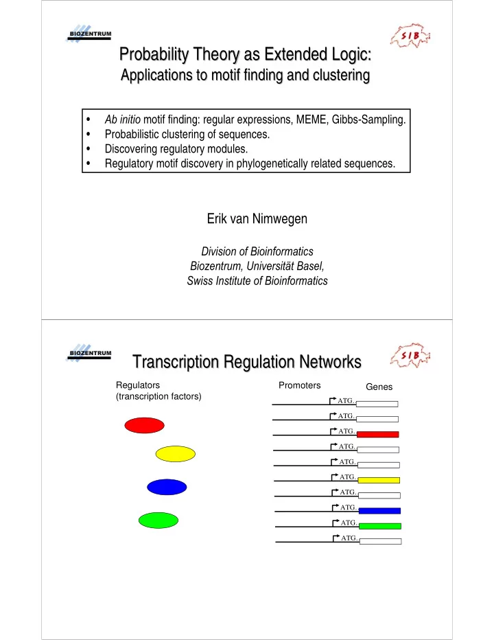
Transcription Regulation Networks Transcription Regulation Networks
ATG….. ATG….. ATG….. ATG….. ATG….. ATG….. ATG….. ATG….. ATG….. ATG…..
Genes Promoters Regulators (transcription factors)