Probability and Statistics for Computer Science Its straigh,orward - - PowerPoint PPT Presentation

ì

Probability and Statistics for Computer Science

“It’s straigh,orward to link a number to the outcome of an

• experiment. The result is a

Random variable.” ---Prof. Forsythe Random variable is a funcDon, it is not the same as in X = X+1

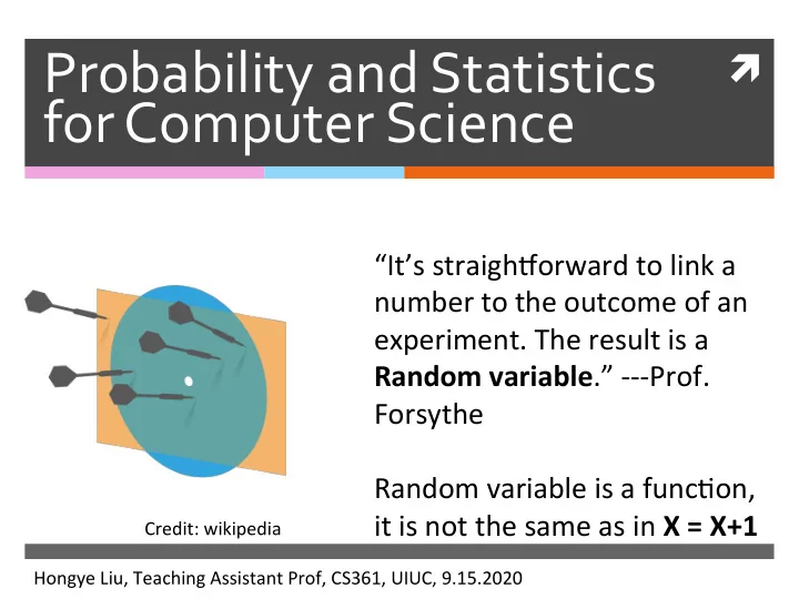
Hongye Liu, Teaching Assistant Prof, CS361, UIUC, 9.15.2020 Credit: wikipedia

Which is larger?

6 The probability of drawing

hands of

5- cards that

have

no pairs

②

0 . 5 ( ng replacement)

> 0.5

A

O is

larger

B

Or

is

larger

g- permit

52×48484×40×36

*

'

Int III

:

Last time

P ( Al B) = Pc An B )

¥

Conditional probability

* Product

rule

• f

joint prob.

* Bayes rule

peal BE PCA

)

* Independence

PLANB)

Objectives

Random

variable

Interface

btw

North .

CS

and

the

* Definition

moi

* probability distribution PDF

CDF

* Conditional probability

distr:

Random numbers

Amount of money on a bet Age at reDrement of a populaDon Rate of vehicles passing by the toll Body temperature of a puppy in its pet clinic Level of the intensity of pain in a toothache

Degree

• f

node

in

network

• ~

Random variable as vectors

• A. McDonald et al. NeuroImage doi: 10.1016/

j.neuroimage.2016.10.048

Brain imaging

• f Human

emoDons A) Moral conflict B) MulD-task C) Rest field

⇐

( A)

CB)

( C)

ily ter

' 774

t,

Random variables

A

random

variable maps

all

• utcomes

eo

Numbers ,

so

( W ) CK )

Bernoulli

it's

a

function ! !

=

panicky

is head

I

Xcw)

Random variables

The values of a random variable can

be either discrete, con5nuous or mixed.

Discrete Random variables

The range of a discrete random

variable is a countable set of real numbers.

'

Random Variable Example

Number of pairs in a hand of 5 cards

Let a single outcome be the hand of 5 cards Each outcome maps to values in the set of

numbers {0, 1, 2}

w =

= ?

O

2

Random Variable Example

Number of pairs in a hand of 6 cards Let a single outcome be the hand

• f 6 cards

What is the range of values of this

random variable?

O

I ,

2 ,

3

Q: Random Variable

If we roll a 3-sided fair die, and define

random variable U, such that

• A. {-1, 0, 1}
• B. {0, 1}

Ucw )=/ §

side

i

w

is side z

w

is

side

3

what is

the range

• f

X = U2

can

take

Three important facts of Random variables

Random variables have

probability func5ons

Random variables can be

condi5oned on events or other random variables

Random variables have averages

Random variables have probability functions

Let X be a random variable The set of outcomes

is an event with probability X is the random variable is any unique instance that X takes on

P(X = x)

{ w Gr

• =p ( { w it .

3 )

Ko

Probability Distribution

is called the probability

distribuDon for all possible x

is also denoted as or for all values that X can

take, and is 0 everywhere else

The sum of the probability

distribuDon is 1

P(X = x) P(x) P(X = x)

p(x)

P(X = x) ≥ 0

• x

P(x) = 1

Examples of Probability Distributions

I

xcws-4 !

Yw!

ucwutf ?

side : )

? ,

side

apex

• N)

XCW )=UZ

pc×=x ) 73

His .

÷i

.

.

l

xcwkfgqt.r.am

;

• .

pcX=K )

A

I

• 1

2C= 0

xcws-4 !

Ye!

z

pika,

P'*"

=/ ÷

a- =/

x

• therwise

I

2C=0

vowel ?

side :

""

÷÷¥*i÷

.

"""YE

. .

• therwise
• 2C

Cumulative distribution

is called the cumulaDve

distribuDon funcDon of X

is also denoted as is a non-decreasing

funcDon of x

P(X ≤ x)

f(x)

P(X ≤ x) P(X ≤ x)

Probability distribution and cumulative distribution

Give the random variable X,

X

1 1/2

X(ω) =

• 1
• utcome of ω is head
• utcome of ω is tail

p(x)

X

1 1/2 1

f(x)

P(X = x) P(X ≤ x)

• 9¥

Q

What

is

the

value ?

A biased

four

• sided

die

is rolled

• nce

Random variable

X

is defined

be the

down - face value

I

p ( X-

• K ) =/

all others

• p

( Xs 47

→

A)

• . I

C)

• . 2

D)

B)

° -3

I

Functions of Random Variables

V

• f y

site ;

3

x#

"

X

• XHXut

• Q. Are these random variables the same?

xcwrt : Ii:

'awry ; Ya:

Bernoulli

RV

• x ~

• '
• }

in

• j = 2X

,

V = Xt Y

• O

A)

U

and

V

are

the

same

BM u

and

V

are

Not

the

same .

⇐ to , if

v→{ o ,

I, -3

Function of random variables: die example

2 3 4 2 3 4 1 1

Roll 4-sided fair die twice. Define these random variables: X, the values of 1st roll Y, the values of 2nd roll Sum S = X + Y Difference D= X - Y

X Y

Size of Sample Space = ?

4×4=16

Random variable: die example

2 3 4 2 3 4 1 1

Roll 4-sided fair die twice.

X Y

Size of Sample Space = 16

x

P(X = 1) P(Y ≤ 2) P(S = 7) P(D ≤ −1)

= 'T

= 'T

O

Random variable: die example

2 3 4 2 3 4 1 1

X Y

P(S = 7) P(D ≤ −1)

2 3 4 2 3 4 1 1

X Y S = X + Y D = X-Y

2 3 4 5 3 4 5 6 4 5 6 5 6 7 8

• 3 -2
• 1 0
• 2 -1

1

• 1 0

1 2 1 2 3 7

¥ 0

plw . s.t.sc#E7 )

• I

= I

Probability distribution of the sum

• f two random variables

Give the random variable S in the 4-

sided die, whose range is {2,3,4,5,6,7,8}, probability distribuDon of S.

S

2 3 4 5 6 7 8

p(s)

1/16

446

46

=

TG

Probability distribution of the difference of two random variables

Give the random variable D = X-Y,

what is the probability distribu<on of D?

1/16

• 3
• z
• l

l

L

Z

Conditional Probability

The probability of A given B

Credit: Prof. Jeremy Orloff & Jonathan Bloom

P(A|B) = P(A ∩ B) P(B)

P(B) = 0

The “Size” analogy

• x

P(x|y) = 1

Conditional probability distribution

• f random variables

The condiDonal probability distribuDon

• f X given Y is

P(x|y) = P(x, y) P(y) P(y) = 0

Pc x . y l = P C X

• x n 'F- y)

p Cy ) = pc 4- y,

p

CK l y) = P C X ⇒4 7-y )

Get the marginal from joint distri.

We can recover the individual

probability distribuDons from the joint probability distribuDon

P(x) =

• y

P(x, y)

P(y) =

• x

P(x, y)

①

pix.gs=pcY1x)p

Epoxy,

y

• = -2 pcY/x > pox)

Y

= pix)

• 2g

= pie,

Joint probabilities sum to 1

The sum of the joint probability

distribuDon

• y
• x

P(x, y) = 1

r

• a

Joint Probability Example

Tossing a coin twice, we define

random variable X and Y for each toss.

X(ω) =

• 1
• utcome of ω is head
• utcome of ω is tail

Y (ω) =

• 1
• utcome of ω is head
• utcome of ω is tail

Joint probability distribution example

1

X Y

P(x, y)

P(x)

P(y)

1 it

. I

¥4

E

DEE

Joint Probability Example

Now we define Sum S = X + Y, Difference D = X – Y. S takes on values {0,1,2} and D takes on values {-1, 0, 1}

X(ω) =

• 1
• utcome of ω is head
• utcome of ω is tail

Y (ω) =

• 1
• utcome of ω is head
• utcome of ω is tail

Joint Probability Example

X =1 X =0 Y =1 Y =0 Y =1 Y =0

S D

2 1 1 1

• 1

P(s, d) 1st toss 2nd toss Suppose coin is fair, and the tosses are independent

f-S

D=d as

=pc

pcs-s.r-dj-I.cz

t

tutte

y

I

4

°

I

4

pcanbt-PCBIAIPCAI-pcalbgpcB.JP ,"%

Joint probability distribution example

1 2 1

• 1

D S P(s, d)

P(s)

P(d)

0¥

¥

• ¥

¥

I

¥

¥

pest -2

pass

city

D

Independence of random variables

Random variable X and Y are

independent if

In the previous coin toss example Are X and Y independent? Are S and D independent?

P(x, y) = P(x)P(y) for all x and y *

Pcs , D) =p is> PCD

)

for all

S, d

Joint probability distribution example

1

X Y

P(x, y)

P(x)

P(y)

1

1 4 1 4 1 4 1 4 1 2 1 2 1 2 1 2

Joint probability distribution example

1 2 1

• 1

D S

1 4 1 4 1 4 1 4 1 4 1 4

1 2

P(s, d)

P(s)

P(d)

1 4 1 4

1 2

O

• 5=1

,

Cleo

C

pcs=f, d -03=0

S

D

are Not

pcS= ' > Pide)=¥

irdept

Joint probability distribution example

1 2 1

• 1

D S

1 4 1 4 1 4 1 4 1 4 1 4

1 2

P(s, d)

P(s)

P(d)

1 4 1 4

1 2

P(S = 1, D = 0) = P(S = 1)P(D = 0)

Conditional probability distribution example

1 2 1

• 1

D S

P(s|d) = P(s, d) P(d)

1 2 1 2

1 1

Bayes rule for random variable

Bayes rule for events generalizes to

random variables

P(A|B) = P(B|A)P(A) P(B)

P(x|y) = P(y|x)P(x) P(y)

= P(y|x)P(x)

• x P(y|x)P(x)

Total Probability

Conditional probability distribution example

1 2 1

• 1

D S

P(s|d) = P(s, d) P(d)

1 2 1 2

1 1

P(D = −1|S = 1) = P(S = 1|D = −1)P(D = −1) P(S = 1)

1 × 1

4 1 2

=

Assignments

Chapter 4 of the textbook Next Dme: More random variable,

ExpectaDons, Variance

Additional References

Charles M. Grinstead and J. Laurie Snell

"IntroducDon to Probability”

Morris H. Degroot and Mark J. Schervish

"Probability and StaDsDcs”

See you next time

See You!