Probabilistic & Unsupervised Learning Beyond linear-Gaussian and Mixture models
Maneesh Sahani
maneesh@gatsby.ucl.ac.uk
Gatsby Computational Neuroscience Unit, and MSc ML/CSML, Dept Computer Science University College London Term 1, Autumn 2015
Probabilistic & Unsupervised Learning Beyond linear-Gaussian and - - PowerPoint PPT Presentation
Probabilistic & Unsupervised Learning Beyond linear-Gaussian and Mixture models Maneesh Sahani maneesh@gatsby.ucl.ac.uk Gatsby Computational Neuroscience Unit, and MSc ML/CSML, Dept Computer Science University College London Term 1,
Maneesh Sahani
maneesh@gatsby.ucl.ac.uk
Gatsby Computational Neuroscience Unit, and MSc ML/CSML, Dept Computer Science University College London Term 1, Autumn 2015
◮ Factor analysis, principle components analysis, probabilistic PCA.
◮ Factor analysis, principle components analysis, probabilistic PCA. ◮ Linear regression, Gaussian processes.
◮ Factor analysis, principle components analysis, probabilistic PCA. ◮ Linear regression, Gaussian processes. ◮ Mixture of Gaussians, mixture of experts.
◮ Factor analysis, principle components analysis, probabilistic PCA. ◮ Linear regression, Gaussian processes. ◮ Mixture of Gaussians, mixture of experts. ◮ Hidden Markov models, linear-Gaussian state space models.
Models consisting of various combinations of:
◮ Linear Gaussian, ◮ Discrete variables, ◮ Chains and trees (or junction trees),
Gaussian
Adapted from Roweis & Ghahramani (1999). A Unifying Review of Linear Gaussian Models. Neural
Gaussian Mixture of Gaussians (VQ) Factor Analysis (PCA) Discrete Latent (mixture) Linear-Gaussian Latent
Adapted from Roweis & Ghahramani (1999). A Unifying Review of Linear Gaussian Models. Neural
Gaussian Mixture of Gaussians (VQ) Factor Analysis (PCA) Hidden Markov Models Linear Dynam- ical Systems Discrete Latent (mixture) Linear-Gaussian Latent Latent Dynamics
Adapted from Roweis & Ghahramani (1999). A Unifying Review of Linear Gaussian Models. Neural
Gaussian Mixture of Gaussians (VQ) Factor Analysis (PCA) Hidden Markov Models Linear Dynam- ical Systems Mixture of Factor Analysers Mixture
Mixture of LDS Discrete Latent (mixture) Linear-Gaussian Latent Latent Dynamics
Adapted from Roweis & Ghahramani (1999). A Unifying Review of Linear Gaussian Models. Neural
Although these models can be powerful, they are undoubtedly still restrictive. There is a need to go beyond the confines of these structures In this half of the course (and today) we will study:
◮ hierarchical models,
Although these models can be powerful, they are undoubtedly still restrictive. There is a need to go beyond the confines of these structures In this half of the course (and today) we will study:
◮ hierarchical models, ◮ distributed models,
Although these models can be powerful, they are undoubtedly still restrictive. There is a need to go beyond the confines of these structures In this half of the course (and today) we will study:
◮ hierarchical models, ◮ distributed models, ◮ nonlinear models,
Although these models can be powerful, they are undoubtedly still restrictive. There is a need to go beyond the confines of these structures In this half of the course (and today) we will study:
◮ hierarchical models, ◮ distributed models, ◮ nonlinear models, ◮ non-Gaussian models.
Although these models can be powerful, they are undoubtedly still restrictive. There is a need to go beyond the confines of these structures In this half of the course (and today) we will study:
◮ hierarchical models, ◮ distributed models, ◮ nonlinear models, ◮ non-Gaussian models.
and various combinations of these.
Although these models can be powerful, they are undoubtedly still restrictive. There is a need to go beyond the confines of these structures In this half of the course (and today) we will study:
◮ hierarchical models, ◮ distributed models, ◮ nonlinear models, ◮ non-Gaussian models.
and various combinations of these. Whilst sometimes tractable (particularly in corner cases), these models will most often require approximate inference.
Much of the world is neither linear nor Gaussian
500 500 10
10
10
Filter Response Probability
Response histogram Gaussian density
. . . and most interesting structure we would like to learn about is not either.
Many generative processes can be naturally described at different levels of detail.
(e.g. objects, illumination, pose) (e.g. object parts, surfaces) (e.g. edges) (retinal image, i.e. pixels)
Biology seems to have developed hierarchical representations.
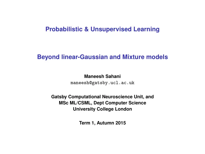
s1 s2 s3 sT x1 x2 x3 xT
Consider a hidden Markov model. To capture N bits of information about the history of the sequence, an HMM requires K = 2N states. In a distributed representation each data point is represented by a vector of (discrete or continous) attibutes. Some attributes might be latent.
◮ For example, consider a model used to predict election outcome. ◮ One might simply assign each voter to one of 4 classes: Labour, Tory, Lib-Dem and
single 4-valued discrete variable.
◮ A better approach might be to model voters using a group of attributes, e.g.:
(Tory, Single, Black, Female, 34 yrs, Urban, Liberal, £35k p.a.).
◮ These attributes resemble factors, but may be discrete (and non-Gaussian), and may
Such distributed representations can be exponentially more efficient than clustering.
Gaussian Mixture of Gaussians (VQ) Factor Analysis (PCA) Hidden Markov Models Linear Dynam- ical Systems Mixture of Factor Analysers Mixture
Mixture of LDS Discrete Latent (mixture) Linear-Gaussian Latent Latent Dynamics
Adapted from Roweis & Ghahramani (1999). A Unifying Review of Linear Gaussian Models. Neural
Gaussian Mixture of Gaussians (VQ) Factor Analysis (PCA) Hidden Markov Models Linear Dynam- ical Systems Mixture of Factor Analysers Mixture
Mixture of LDS Independent Components Analysis Nonlinear Dynamical Systems Discrete Latent (mixture) Linear-Gaussian Latent Latent Dynamics Nonlinear link functions
Adapted from Roweis & Ghahramani (1999). A Unifying Review of Linear Gaussian Models. Neural
Gaussian Mixture of Gaussians (VQ) Factor Analysis (PCA) Hidden Markov Models Linear Dynam- ical Systems Mixture of Factor Analysers Mixture
Mixture of LDS Independent Components Analysis Nonlinear Dynamical Systems Cooperative Vector Quan- tisation Factorial HMM Discrete Latent (mixture) Linear-Gaussian Latent Latent Dynamics Nonlinear link functions Distributed Latent
Adapted from Roweis & Ghahramani (1999). A Unifying Review of Linear Gaussian Models. Neural
Gaussian Mixture of Gaussians (VQ) Factor Analysis (PCA) Hidden Markov Models Linear Dynam- ical Systems Mixture of Factor Analysers Mixture
Mixture of LDS Independent Components Analysis Nonlinear Dynamical Systems Cooperative Vector Quan- tisation Factorial HMM Sigmoid Belief Nets Nonlinear Gaussian Belief Nets Discrete Latent (mixture) Linear-Gaussian Latent Latent Dynamics Nonlinear link functions Distributed Latent Hierarchy
Adapted from Roweis & Ghahramani (1999). A Unifying Review of Linear Gaussian Models. Neural
Sometimes called the cocktail party problem. ?
◮ Given signals from one or more receivers that mix signals from one or more sources,
recover the timeseries of the source signals.
◮ Independent components analysis: assumes that sources are independent and
non-Gaussian.
500 500 10
10
10
Response histogram Gaussian density
−4 −2 2 4 −4 −3 −2 −1 1 2 3 4 5 Mixture of Heavy Tailed Sources −3 −2 −1 1 2 −3 −2 −1 1 2 3 Mixture of Light Tailed Sources
These distributions are gen- erated by linearly combining (or mixing) two non-Gaussian sources.
◮ The ICA graphical model is identical to factor analysis:
xd =
K
Λdk yk + ǫd
with yk ∼ Py non-Gaussian.
x1 x2 xD y1 y2 yK
Differences:
◮ Well-posed even with K ≥ D (e.g., K = D = 2 above). ◮ With non-zero noise, MAP inference is non-linear, and the full posterior is non-Gaussian. ◮ This makes making exact inference and learning difficult for most Py.
◮ The special case of K = D, and zero observation noise has been studied extensively
(standard infomax ICA, c.f. PCA): x = Λy which implies y = Wx where W = Λ−1 where y are the independent components (factors), x are the observations, and W is the unmixing matrix.
◮ The special case of K = D, and zero observation noise has been studied extensively
(standard infomax ICA, c.f. PCA): x = Λy which implies y = Wx where W = Λ−1 where y are the independent components (factors), x are the observations, and W is the unmixing matrix.
◮ The likelihood can be obtained by transforming the density of y to that of x. If F : y → x
is a differentiable bijection, and if dy is a small neighbourhood around y, then Px(x)dx = Py(y)dy = Py(F −1(x))
dx
dx
◮ This gives (for parameter W):
P(x|W) = |W|
Py([Wx]k
yk
)
where py is marginal probability distribution of factors.
◮ Consider a feedforward model:
yi = Wix; zi = fi(yi) with a monotonic squashing function fi(−∞) = 0, fi(+∞) = 1.
◮ Consider a feedforward model:
yi = Wix; zi = fi(yi) with a monotonic squashing function fi(−∞) = 0, fi(+∞) = 1.
◮ Infomax finds filtering weights W maximizing the information carried by z about x:
argmax
W
I(x; z) = argmax
W
H(z) − H(z|x) = argmax
W
H(z) Thus we just have to maximize entropy of z: make it as uniform as possible on [0, 1] (note squashing function).
◮ But if data were generated from a square noiseless causal ICA then best we can do is if
zi = fi(yi) = cdfi(yi) and W = Λ−1 Infomax ICA ⇔ square noiseless causal ICA.
◮ Another view: redundancy reduction in the representation z of the data x.
argmax
W
H(z) = argmax
W
H(zi) − I(z1, . . . , zD) See: MacKay (1996), Pearlmutter and Parra (1996), Cardoso (1997) for equivalence, Teh et al (2003) for an energy-based view.
◮ Log likelihood of data:
log P(x) = log |W| +
log Py(Wix)
◮ Log likelihood of data:
log P(x) = log |W| +
log Py(Wix)
◮ Learning by gradient ascent:
∆W ∝ ∇W = W −T + g(y)xT
g(y) = ∂ log Py(y)
∂y
◮ Log likelihood of data:
log P(x) = log |W| +
log Py(Wix)
◮ Learning by gradient ascent:
∆W ∝ ∇W = W −T + g(y)xT
g(y) = ∂ log Py(y)
∂y
◮ Better approach: natural gradient
∆W ∝ ∇W(W TW) = W + g(y)yTW
(see MacKay 1996).
◮ Log likelihood of data:
log P(x) = log |W| +
log Py(Wix)
◮ Learning by gradient ascent:
∆W ∝ ∇W = W −T + g(y)xT
g(y) = ∂ log Py(y)
∂y
◮ Better approach: natural gradient
∆W ∝ ∇W(W TW) = W + g(y)yTW
(see MacKay 1996).
◮ Note: we can’t use EM in the square noiseless causal ICA model. Why?
The kurtosis (or excess kurtosis) measures how “peaky” or “heavy-tailed” a distribution is: K = E((x − µ)4) E((x − µ)2)2 − 3, where µ = E(x) is the mean of x. Gaussian distributions have zero kurtosis. Heavy tailed: positive kurtosis (leptokurtic). Light tailed: negative kurtosis (platykurtic). Some ICA algorithms are essentially kurtosis pursuit approaches. Possibly fewer assumptions about generating distributions.
Applications:
◮ Separating auditory sources ◮ Analysis of EEG data ◮ Analysis of functional MRI data ◮ Natural scene analysis ◮ . . .
Extensions:
◮ Non-zero output noise – approximate posteriors and learning. ◮ Undercomplete (K < D) or overcomplete (K > D). ◮ Learning prior distributions (on y). ◮ Dynamical hidden models (on y). ◮ Learning number of sources. ◮ Time-varying mixing matrix. ◮ Nonparametric, kernel ICA. ◮ . . .
?
◮ ICA solution to blind source separation assumes no dependence across time; still works
fine much of the time.
◮ Many other algorithms: DCA, SOBI, JADE, . . .
Olshausen & Field (1996)
y1 y2 y3 yT x1 x2 x3 xT u1 u2 u3 uT
f f f f g g g g
yt+1 = f(yt, ut) + wt xt = g(yt, ut) + vt wt, vt usually still Gaussian. yt f(yt)
y1 y2 y3 yT x1 x2 x3 xT u1 u2 u3 uT
f f f f g g g g
yt+1 = f(yt, ut) + wt xt = g(yt, ut) + vt wt, vt usually still Gaussian. Extended Kalman Filter (EKF): linearise nonlinear functions about current estimate, ˆ yt
t:
yt+1 ≈ f(ˆ yt
t, ut) + ∂f
∂yt
yt
t
(yt − ˆ
yt
t) + wt
xt ≈ g(ˆ yt−1
t
, ut) + ∂g ∂yt
yt−1
t
(yt − ˆ
yt−1
t
) + vt
yt f(yt)
ˆ
yt
t
y1 y2 y3 yT x1 x2 x3 xT u1 u2 u3 uT
yt+1 = f(yt, ut) + wt xt = g(yt, ut) + vt wt, vt usually still Gaussian. Extended Kalman Filter (EKF): linearise nonlinear functions about current estimate, ˆ yt
t:
yt+1 ≈ f(ˆ yt
t, ut)
+ ∂f ∂yt
yt
t
(yt − ˆ
yt
t) + wt
xt ≈ g(ˆ yt−1
t
, ut)
+ ∂g ∂yt
yt−1
t
(yt − ˆ
yt−1
t
) + vt
yt f(yt)
ˆ
yt
t
Run the Kalman filter (smoother) on non-stationary linearised system ( At, Bt, Ct, Dt):
◮ Adaptively approximates non-Gaussian messages by Gaussians.
y1 y2 y3 yT x1 x2 x3 xT u1 u2 u3 uT
yt+1 = f(yt, ut) + wt xt = g(yt, ut) + vt wt, vt usually still Gaussian. Extended Kalman Filter (EKF): linearise nonlinear functions about current estimate, ˆ yt
t:
yt+1 ≈ f(ˆ yt
t, ut)
+ ∂f ∂yt
yt
t
(yt − ˆ
yt
t) + wt
xt ≈ g(ˆ yt−1
t
, ut)
+ ∂g ∂yt
yt−1
t
(yt − ˆ
yt−1
t
) + vt
yt f(yt)
ˆ
yt
t
Run the Kalman filter (smoother) on non-stationary linearised system ( At, Bt, Ct, Dt):
◮ Adaptively approximates non-Gaussian messages by Gaussians. ◮ Local linearisation depends on central point of distribution ⇒ approximation degrades
with increased state uncertainty.
y1 y2 y3 yT x1 x2 x3 xT u1 u2 u3 uT
yt+1 = f(yt, ut) + wt xt = g(yt, ut) + vt wt, vt usually still Gaussian. Extended Kalman Filter (EKF): linearise nonlinear functions about current estimate, ˆ yt
t:
yt+1 ≈ f(ˆ yt
t, ut)
+ ∂f ∂yt
yt
t
(yt − ˆ
yt
t) + wt
xt ≈ g(ˆ yt−1
t
, ut)
+ ∂g ∂yt
yt−1
t
(yt − ˆ
yt−1
t
) + vt
yt f(yt)
ˆ
yt
t
Run the Kalman filter (smoother) on non-stationary linearised system ( At, Bt, Ct, Dt):
◮ Adaptively approximates non-Gaussian messages by Gaussians. ◮ Local linearisation depends on central point of distribution ⇒ approximation degrades
with increased state uncertainty. May work acceptably for close-to-linear systems.
y1 y2 y3 yT x1 x2 x3 xT u1 u2 u3 uT
yt+1 = f(yt, ut) + wt xt = g(yt, ut) + vt wt, vt usually still Gaussian. Extended Kalman Filter (EKF): linearise nonlinear functions about current estimate, ˆ yt
t:
yt+1 ≈ f(ˆ yt
t, ut)
+ ∂f ∂yt
yt
t
(yt − ˆ
yt
t) + wt
xt ≈ g(ˆ yt−1
t
, ut)
+ ∂g ∂yt
yt−1
t
(yt − ˆ
yt−1
t
) + vt
yt f(yt)
ˆ
yt
t
Run the Kalman filter (smoother) on non-stationary linearised system ( At, Bt, Ct, Dt):
◮ Adaptively approximates non-Gaussian messages by Gaussians. ◮ Local linearisation depends on central point of distribution ⇒ approximation degrades
with increased state uncertainty. May work acceptably for close-to-linear systems. Can base EM-like algorithm on EKF/EKS (or alternatives).
Nonlinear message passing can also be used to implement online parameter learning in (non)linear latent state-space systems:
Nonlinear message passing can also be used to implement online parameter learning in (non)linear latent state-space systems: Eg: for linear model, augment state vector to include the model parameters :
=
yt =
yt A C
,
and introduce nonlinear transition
=
f and output map
=
g:
=
yt+1 =
=
f (
=
yt) +
=
wt
=
f
yt A C
=
Ayt A C
;
=
wt =
wt
xt =
=
g(
=
yt) + vt
=
g
yt A C
= Cyt
(where A and C need to be vectorised and de-vectorised as appropriate).
Nonlinear message passing can also be used to implement online parameter learning in (non)linear latent state-space systems: Eg: for linear model, augment state vector to include the model parameters :
=
yt =
yt A C
,
and introduce nonlinear transition
=
f and output map
=
g:
=
yt+1 =
=
f (
=
yt) +
=
wt
=
f
yt A C
=
Ayt A C
;
=
wt =
wt
xt =
=
g(
=
yt) + vt
=
g
yt A C
= Cyt
(where A and C need to be vectorised and de-vectorised as appropriate). Use EKF to compute online estimates of E[
=
yt|x1, . . . , xt] and Cov[
=
yt|x1, . . . , xt]. These now include mean and posterior variance of parameter estimates.
◮ Pseudo-Bayesian approach: gives Gaussian distributions over parameters.
Nonlinear message passing can also be used to implement online parameter learning in (non)linear latent state-space systems: Eg: for linear model, augment state vector to include the model parameters :
=
yt =
yt A C
,
and introduce nonlinear transition
=
f and output map
=
g:
=
yt+1 =
=
f (
=
yt) +
=
wt
=
f
yt A C
=
Ayt A C
;
=
wt =
wt
xt =
=
g(
=
yt) + vt
=
g
yt A C
= Cyt
(where A and C need to be vectorised and de-vectorised as appropriate). Use EKF to compute online estimates of E[
=
yt|x1, . . . , xt] and Cov[
=
yt|x1, . . . , xt]. These now include mean and posterior variance of parameter estimates.
◮ Pseudo-Bayesian approach: gives Gaussian distributions over parameters. ◮ Can model nonstationarity by assuming non-zero innovations noise in A, C.
Nonlinear message passing can also be used to implement online parameter learning in (non)linear latent state-space systems: Eg: for linear model, augment state vector to include the model parameters :
=
yt =
yt A C
,
and introduce nonlinear transition
=
f and output map
=
g:
=
yt+1 =
=
f (
=
yt) +
=
wt
=
f
yt A C
=
Ayt A C
;
=
wt =
wt
xt =
=
g(
=
yt) + vt
=
g
yt A C
= Cyt
(where A and C need to be vectorised and de-vectorised as appropriate). Use EKF to compute online estimates of E[
=
yt|x1, . . . , xt] and Cov[
=
yt|x1, . . . , xt]. These now include mean and posterior variance of parameter estimates.
◮ Pseudo-Bayesian approach: gives Gaussian distributions over parameters. ◮ Can model nonstationarity by assuming non-zero innovations noise in A, C. ◮ Not simple to implement for Q and R (e.g. covariance constraints?).
Nonlinear message passing can also be used to implement online parameter learning in (non)linear latent state-space systems: Eg: for linear model, augment state vector to include the model parameters :
=
yt =
yt A C
,
and introduce nonlinear transition
=
f and output map
=
g:
=
yt+1 =
=
f (
=
yt) +
=
wt
=
f
yt A C
=
Ayt A C
;
=
wt =
wt
xt =
=
g(
=
yt) + vt
=
g
yt A C
= Cyt
(where A and C need to be vectorised and de-vectorised as appropriate). Use EKF to compute online estimates of E[
=
yt|x1, . . . , xt] and Cov[
=
yt|x1, . . . , xt]. These now include mean and posterior variance of parameter estimates.
◮ Pseudo-Bayesian approach: gives Gaussian distributions over parameters. ◮ Can model nonstationarity by assuming non-zero innovations noise in A, C. ◮ Not simple to implement for Q and R (e.g. covariance constraints?). ◮ May be faster than EM/gradient approaches.
Sometimes called the joint-EKF approach.
Undirected graphical model (i.e. a Markov network) over a vector of binary variables si ∈ {0, 1}. Some variables may be hidden, some may be visible (observed). P(s|W, b) = 1 Z exp
Wijsisj −
bisi
Learning algorithm: a gradient version of EM
◮ E step involves computing averages w.r.t. P(sH|sV, W, b) (“clamped phase”). This could
be done either exactly or (more usually) approximately using Gibbs sampling or loopy BP .
◮ The M step requires gradients w.r.t. Z, which can be computed by averages w.r.t.
P(s|W, b) (“unclamped phase”).
∇Wij = sisjc − sisju
log P(sVsH|W, b) =
Wijsisj −
bisi − log Z with Z =
s e
i bi si
Generalised (gradient M-step) EM requires parameter step
∆Wij ∝ ∂ ∂Wij
Write c (clamped) for expectations under P(s|sV) (with P(sV|sV) = 1). Then
∇Wij = ∂ ∂Wij
i bisic − log Z
∂ ∂Wij
log Z
= sisjc − 1
Z
∂ ∂Wij
e
i bi si
= sisjc −
1 Z e
i bi si sisj
= sisjc −
P(s|W, b)sisj
= sisjc − sisju
with u (unclamped) an expectation under the current joint distribution.
Directed graphical model (i.e. a Bayesian network) over a vector of binary variables si ∈ {0, 1}. P(s|W, b) =
P(si|{sj}j<i, W, b) P(si = 1|{sj}j<i, W, b) = 1 1 + exp{−
j<i Wijsj − bi} ◮ parents most often grouped into layers ◮ logistic function of linear combination of parents ◮ “generative multilayer perceptron” (“neural network”)
Learning algorithm: a gradient version of EM
◮ E step involves computing averages w.r.t. P(sH|sV, W, b). This could be done either
exactly or approximately using Gibbs sampling or mean field approximations. Or using a parallel ‘recognition network’ (the Helmholtz machine).
◮ Unlike Boltzmann machines, there is no partition function, so no need for an unclamped
phase in the M step.
s(1)
1
s(1)
2
s(1)
3
s(1)
T
s(2)
1
s(2)
2
s(2)
3
s(2)
T
s(3)
1
s(3)
2
s(3)
3
s(3)
T
x1 x2 x3 xT
◮ Hidden Markov models with many state variables (i.e. distributed state representation). ◮ Each state variable evolves independently. ◮ The state can capture many bits of information about the sequence (linear in the number
◮ E step is typically intractable (due to explaining away in latent states).
◮ Distributed HMM with structured dependencies amongst latent states.
Topic modelling: given a corpus of documents, find the “topics” they discuss.
Topic modelling: given a corpus of documents, find the “topics” they discuss. Example: consider abstracts of papers PNAS.
Global climate change and mammalian species diversity in U.S. national parks National parks and bioreserves are key conservation tools used to protect species and their habitats within the confines of fixed political boundaries. This inflexibility may be their ”Achilles’ heel” as conservation tools in the face of emerging global-scale environmental problems such as climate change. Global climate change, brought about by rising levels of greenhouse gases, threatens to alter the geographic distribution of many habitats and their component species.... The influence of large-scale wind power on global climate Large-scale use of wind power can alter local and global climate by extracting kinetic energy and altering turbulent transport in the atmospheric boundary layer. We report climate-model simulations that address the possible climatic impacts of wind power at regional to global scales by using two general circulation models and several parameterizations of the interaction of wind turbines with the boundary layer.... Twentieth century climate change: Evidence from small glaciers The relation between changes in modern glaciers, not including the ice sheets of Greenland and Antarctica, and their climatic environment is investigated to shed light on paleoglacier evidence of past climate change and for projecting the effects of future climate warming on cold regions of the world. Loss of glacier volume has been more or less continuous since the 19th century, but it is not a simple adjustment to the end of an ”anomalous” Little Ice Age....
Example topics discovered from PNAS abstracts (each topic represented in terms of the top 5 most common words in that topic).
Recall the Bayesian coin toss example. P(H|q) = q P(T|q) = 1 − q The probability of a sequence of coin tosses is: P(HHTT · · · HT|q) = q#heads(1 − q)#tails A conjugate prior for q is the Beta distribution: P(q) = Γ(a + b)
Γ(a)Γ(b)qa−1(1 − q)b−1
a, b ≥ 0
0.1 0.2 0.3 0.4 0.5 0.6 0.7 0.8 0.9 1 0.5 1 1.5 2 2.5
q P(q)
Imagine a Bayesian dice throwing example. P(1|q) = q1 P(2|q) = q2 P(3|q) = q3 P(4|q) = q4 P(5|q) = q5 P(6|q) = q6 with qi ≥ 0,
i qi = 1.
Imagine a Bayesian dice throwing example. P(1|q) = q1 P(2|q) = q2 P(3|q) = q3 P(4|q) = q4 P(5|q) = q5 P(6|q) = q6 with qi ≥ 0,
i qi = 1. The probability of a sequence of dice throws is:
P(34156 · · · 12|q) =
6
q# face i
i
Imagine a Bayesian dice throwing example. P(1|q) = q1 P(2|q) = q2 P(3|q) = q3 P(4|q) = q4 P(5|q) = q5 P(6|q) = q6 with qi ≥ 0,
i qi = 1. The probability of a sequence of dice throws is:
P(34156 · · · 12|q) =
6
q# face i
i
A conjugate prior for q is the Dirichlet distribution: P(q) = Γ(
i ai)
qai−1
i
qi ≥ 0,
i qi = 1
ai ≥ 0
Dirichlet [1,1,1] q1 q2 Dirichlet [2,2,2] q1 q2 Dirichlet [2,10,2] q1 q2 Dirichlet [0.9,0.9,0.9] q1 q2Each document is a sequence of words, we model it using a mixture model by ignoring the sequential nature—“bag-of-words” assumption.
Each document is a sequence of words, we model it using a mixture model by ignoring the sequential nature—“bag-of-words” assumption.
document d=1...D
◮ For each document:
Each document is a sequence of words, we model it using a mixture model by ignoring the sequential nature—“bag-of-words” assumption. xid
word i=1...Nd document d=1...D
◮ For each document:
◮ generate words iid:
Each document is a sequence of words, we model it using a mixture model by ignoring the sequential nature—“bag-of-words” assumption. xid zid
word i=1...Nd document d=1...D
φk
◮ For each document:
◮ generate words iid: ◮ draw word from a topic-specific dist:
xid ∼ Discrete(φzid )
Each document is a sequence of words, we model it using a mixture model by ignoring the sequential nature—“bag-of-words” assumption. xid zid
word i=1...Nd
θd
document d=1...D
φk
◮ For each document:
◮ generate words iid: ◮ draw topic from a document-specific dist:
zid ∼ Discrete(θd)
◮ draw word from a topic-specific dist:
xid ∼ Discrete(φzid )
Each document is a sequence of words, we model it using a mixture model by ignoring the sequential nature—“bag-of-words” assumption. xid zid
word i=1...Nd
θd α
document d=1...D
φk
◮ For each document:
◮ draw a distribution over topics
θd ∼ Dir(α, . . . , α)
◮ generate words iid: ◮ draw topic from a document-specific dist:
zid ∼ Discrete(θd)
◮ draw word from a topic-specific dist:
xid ∼ Discrete(φzid )
Each document is a sequence of words, we model it using a mixture model by ignoring the sequential nature—“bag-of-words” assumption. xid zid
word i=1...Nd
θd α
document d=1...D
φk
topic k=1...K
β
◮ Draw topic distributions from a prior
φk ∼ Dir(β, . . . , β)
◮ For each document:
◮ draw a distribution over topics
θd ∼ Dir(α, . . . , α)
◮ generate words iid: ◮ draw topic from a document-specific dist:
zid ∼ Discrete(θd)
◮ draw word from a topic-specific dist:
xid ∼ Discrete(φzid ) Multiple mixtures of discrete distributions, sharing the same set of components (topics).
Let Ndw be the number of times word w appears in document d, and Pdw is the probability of word w appearing in document d. p(N|P) =
P
Ndw dw
likelihood term Pdw =
p(pick topic k)p(pick word w|k) =
K
θdkφkw
Pdw
= θdk · φkw
This decomposition is similar to PCA and factor analysis, but not Gaussian. Related to non-negative matrix factorisation (NMF).
◮ Exact inference in latent Dirichlet allocation is intractable, and typically either variational
◮ Latent Dirichlet allocation is an example of a mixed membership model from statistics. ◮ Latent Dirichlet allocation has also been applied to computer vision, social network
modelling, natural language processing. . .
◮ Generalizations:
◮ Relax the bag-of-words assumption (e.g. a Markov model). ◮ Model changes in topics through time. ◮ Model correlations among occurrences of topics. ◮ Model authors, recipients, multiple corpora. ◮ Cross modal interactions (images and tags). ◮ Nonparametric generalisations.
We can see matrix factorisation methods as performing linear dimensionaliy reduction. There are many ways to generalise PCA and FA to deal with data which lie on a nonlinear manifold:
◮ Nonlinear autoencoders ◮ Generative topographic mappings (GTM) and Kohonen self-organising maps (SOM) ◮ Multi-dimensional scaling (MDS) ◮ Kernel PCA (based on MDS representation) ◮ Isomap ◮ Locally linear embedding (LLE) ◮ Stochastic Neighbour Embedding ◮ Gaussian Process Latent Variable Models (GPLVM)
We have viewed PCA as providing a decomposition of the covariance or scatter matrix S. We
minimise
E =
(Gij − yi · yj)2
for y ∈ Rk. That is, look for a k-dimensional embedding in which dot products (which depend on lengths, and angles) are preserved as well as possible. We will see that this is also equivalent to preserving distances between points.
Consider the eigendecomposition of G: G = UΛUT arranged so
λ1 ≥ · · · ≥ λm ≥ 0
The best rank-k approximation G ≈ Y TY is given by: Y T = [U]1:m,1:k[Λ1/2]1:k,1:k;
= [UΛ1/2]1:m,1:k
Y = [Λ1/2UT]1:k,1:m
√λ1 uT
1
√λ2 uT
2
. . .
√λk uT
k
. . .
√λm uT
m
Consider the eigendecomposition of G: G = UΛUT arranged so
λ1 ≥ · · · ≥ λm ≥ 0
The best rank-k approximation G ≈ Y TY is given by: Y T = [U]1:m,1:k[Λ1/2]1:k,1:k;
= [UΛ1/2]1:m,1:k
Y = [Λ1/2UT]1:k,1:m
√λ1 uT
1
√λ2 uT
2
. . .
√λk uT
k
. . .
√λm uT
m
y1 y2
· · ·
ym
Consider the eigendecomposition of G: G = UΛUT arranged so
λ1 ≥ · · · ≥ λm ≥ 0
The best rank-k approximation G ≈ Y TY is given by: Y T = [U]1:m,1:k[Λ1/2]1:k,1:k;
= [UΛ1/2]1:m,1:k
Y = [Λ1/2UT]1:k,1:m
√λ1 uT
1
√λ2 uT
2
. . .
√λk uT
k
. . .
√λm uT
m
y1 y2
· · ·
ym The same operations can be performed on the kernel Gram matrix ⇒ Kernel PCA.
Suppose all we were given were distances or symmetric “dissimilarities” ∆ij.
∆ = ∆12 ∆13 ∆14 ∆12 ∆23 ∆24 ∆13 ∆23 ∆34 ∆14 ∆24 ∆34
Goal: Find vectors yi such that yi − yj ≈ ∆ij. This is called Multidimensional Scaling (MDS).
Assume the dissimilarities represent Euclidean distances between points in some high-D space.
∆ij = xi − xj with
xi = 0. We have:
∆2
ij = xi2 + xj2 − 2xi · xj
∆2
ik = mxi2 +
xk2 − 0
∆2
kj =
xk2 + mxj2 − 0
∆2
kl = 2m
xk2 ⇒ Gij = xi · xj = 1
2
m
(∆2
ik + ∆2 kj) − 1
m2
∆2
kl − ∆2 ij
We will actually minimize the error in the dot products:
E =
(Gij − yi · yj)2
As in PCA, this is given by the top slice of the eigenvector matrix.
√λ1 uT
1
√λ2 uT
2
. . .
√λk uT
k
. . .
√λm uT
m
y1 y2
· · ·
ym
G = 1 2
m (∆21 + 1∆2) − ∆2 − 1 m2 1T∆21
Y = [Λ1/2UT]1:k,1:m
(1 is a matrix of ones.)
◮ Eigenvectors. Ordered, scaled and truncated to yield low-dimensional embedded
points yi.
◮ Eigenvalues. Measure how much each dimension contributes to dot products. ◮ Estimated dimensionality. Number of significant (nonnegative – negative possible if
∆ij are not metric) eigenvalues.
Dual matrices: S = 1 m XX T scatter matrix
(n × n)
G = X TX Gram matrix
(m × m)
◮ Same eigenvalues up to a constant factor. ◮ Equivalent on metric data, but MDS can run on non-metric dissimilarities. ◮ Computational cost is different.
◮ PCA: O((m + k)n2) ◮ MDS: O((n + k)m2)
MDS can be generalised to permit a monotonic mapping:
∆ij → g(∆ij),
even if this violates metric rules (like the triangle inequality). This can introduce a non-linear warping of the manifold.
Idea: try to trace distance along the manifold. Use geodesic instead of (transformed) Euclidean distances in MDS.
◮ preserves local structure ◮ estimates “global” structure ◮ preserves information (MDS)
manifold). Euclidean distances are preserved within a neighbourhood.
within neighbourhoods.
First we construct a graph linking each point to its neighbours.
◮ vertices represent input points ◮ undirected edges connect neighbours (weight = Euclidean distance)
Forms a discretised approximation to the submanifold, assuming:
◮ Graph is singly-connected. ◮ Graph neighborhoods reflect manifold neighborhoods. No “short cuts”.
Defining the neighbourhood is critical: k-nearest neighbours, inputs within a ball of radius r, prior knowledge.
Estimate distances by shortest path in graph.
∆ij =
min
path(xi,xj)
δi
◮ Better estimates for denser sampling. ◮ Short cuts very dangerous (“average” path distance?) .
Embed using metric MDS (path distances obey the triangle inequality)
◮ Eigenvectors of Gram matrix yield low-dimensional embedding. ◮ Number of significant eigenvalues estimates dimensionality.
MDS and isomap preserve local and global (estimated, for isomap) distances. PCA preserves local and global structure. Idea: estimate local (linear) structure of manifold. Preserve this as well as possible.
◮ preserves local structure (not just distance) ◮ not explicitly global ◮ preserves only local information
Just as in isomap, we first define neighbouring points for each input. Equivalent to the isomap graph, but we won’t need the graph structure. Forms a discretised approximation to the submanifold, assuming:
◮ Graph is singly-connected — although will “work” if not. ◮ Neighborhoods reflect manifold neighborhoods. No “short cuts”.
Defining the neighbourhood is critical: k-nearest neighbours, inputs within a ball of radius r, prior knowledge.
Estimate local weights to minimize error
Φ(W) =
Wijxj
Wij = 1
◮ Linear regression – under- or over-constrained depending on |Ne(i)|. ◮ Local structure – optimal weights are invariant to rotation, translation and scaling. ◮ Short cuts less dangerous (one in many).
Minimise reconstruction errors in y-space under the same weights:
ψ(Y) =
Wijyj
subject to:
yi = 0;
yiyT
i = mI
We can re-write the cost function in quadratic form:
ψ(Y) =
Ψij[Y TY]ij with Ψ = (I − W)T(I − W)
Minimise by setting Y to equal the bottom 2 . . . k + 1 eigenvectors of Ψ. (Bottom eigenvector always 1 – discard due to centering constraint)
Many similarities
◮ Graph-based, spectral methods ◮ No local optima
Essential differences
◮ LLE does not estimate dimensionality ◮ Isomap can be shown to be consistent; no theoretical guarantees for LLE. ◮ LLE diagonalises a sparse matrix – more efficient than isomap. ◮ Local weights vs. local & global distances.
Unfold neighbourhood graph preserving local structure.
i yj. Then:
Maximise Tr [K] subject to:
(centered) K 0 (positive definite) Kii − 2Kij + Kjj
= xi − xj2 for j ∈ Ne(i)
(locally metric) This is a semi-definite program: convex optimisation with unique solution.
Softer “probabilistic” notions of neighbourhood and consistency. High-D “transition” probabilities: pj|i = e− 1
2 xi−xj2/σ2
2 xi−xk 2/σ2
for j = i, pi|i = 0 Find {yi} ⊂ Rk to: minimise
pj|i log pj|i qj|i with qj|i = e− 1
2 yi−yj2
2 yi−yk 2 .
Nonconvex optimisation is initialisation dependent. Scale σ plays a similar role to neighbourhood definition:
◮ Fixed σ: resembles a fixed-radius ball. ◮ Choose σi to maintain consistent entropy in pj|i of log2 k: similar to k-nearest
neighbours.
◮ Symmetrise probabilities (pij = pji)
pij = e− 1
2 xi−xj2/σ2
2 xl−xk 2/σ2
for j = i
◮ Gaussian Process Latent Variable Models. Lawrence. Advances in Neural Information
Processing Systems, 2004. Define qij analagously, optimise joint KL.
◮ Heavy-tailed embedding distributions allow embedding to lower dimensions than true
manifold: qij =
(1 + yi − yj2)−1
Student-t distribution defines “t-SNE”. Focus is on visualisation, rather than manifold discovery.
Recap: probabilistic PCA yi|xi, Λ ∼ N(Λxi, β−1I) xi ∼ N(0, I)
Recap: probabilistic PCA yi|xi, Λ ∼ N(Λxi, β−1I) xi ∼ N(0, I) Usually: compute posterior over X = [x1, . . . , xN]⊤, maximizing likelihood over Λ.
Recap: probabilistic PCA yi|xi, Λ ∼ N(Λxi, β−1I) xi ∼ N(0, I) Usually: compute posterior over X = [x1, . . . , xN]⊤, maximizing likelihood over Λ. Suppose we know the values of the latent X, then we can integrate out Λ (c.f. linear regression), giving a conditional probability of Y = [y1 . . . yN]⊤:
Λ ∼ N(0, α−1I)
p(Y|X) ∼ |2πK|− D
2 exp
2Tr[K −1YY ⊤]
This is just D independent Gaussian processes, one for each dimension of Y! Each Gaussian process describes a mapping from latent space x to one dimension of y.
Recap: probabilistic PCA yi|xi, Λ ∼ N(Λxi, β−1I) xi ∼ N(0, I) Usually: compute posterior over X = [x1, . . . , xN]⊤, maximizing likelihood over Λ. Suppose we know the values of the latent X, then we can integrate out Λ (c.f. linear regression), giving a conditional probability of Y = [y1 . . . yN]⊤:
Λ ∼ N(0, α−1I)
p(Y|X) ∼ |2πK|− D
2 exp
2Tr[K −1YY ⊤]
This is just D independent Gaussian processes, one for each dimension of Y! Each Gaussian process describes a mapping from latent space x to one dimension of y. Replacing the linear kernel with nonlinear kernels gives nonlinear mappings—nonlinear dimensionality reduction.
Recap: probabilistic PCA yi|xi, Λ ∼ N(Λxi, β−1I) xi ∼ N(0, I) Usually: compute posterior over X = [x1, . . . , xN]⊤, maximizing likelihood over Λ. Suppose we know the values of the latent X, then we can integrate out Λ (c.f. linear regression), giving a conditional probability of Y = [y1 . . . yN]⊤:
Λ ∼ N(0, α−1I)
p(Y|X) ∼ |2πK|− D
2 exp
2Tr[K −1YY ⊤]
This is just D independent Gaussian processes, one for each dimension of Y! Each Gaussian process describes a mapping from latent space x to one dimension of y. Replacing the linear kernel with nonlinear kernels gives nonlinear mappings—nonlinear dimensionality reduction. But now dependence on X is complicated—instead of computing a posterior over X we can
For many probabilistic models of interest, exact inference is not computationally feasible. This occurs for three (main) reasons:
◮ Distributions may have complicated forms (e.g. non-linearities in generative model). ◮ “Explaining away” causes coupling from observations
Observing the value of a child induces dependencies amongst its parents. x1 y1 y2 yK
◮ Even with simple models, being Bayesian and computing the full posterior over both
latent variables and parameters There is often strong coupling between latent variables and parameters. We can still work with such models by using approximate inference techniques to estimate the latent variables.
◮ Linearisation: Approximate nonlinearities by Taylor series expansion about a point (e.g.
the approximate mean or mode of the hidden variable distribution). Linear approximations are particularly useful since Gaussian distributions are closed under linear transformations (e.g., EKF). Also Laplace’s approximation.
◮ Monte Carlo Sampling: Approximate posterior distribution over unobserved variables by
a set of random samples. We often need Markov chain Monte carlo or sequential Monte Carlo methods to sample from difficult distributions.
◮ Variational Methods: Approximate the hidden variable posterior p(H) with a tractable
form q(H), such that KL[qp] is minimised. This gives a lower bound on the likelihood that can be maximised with respect to the parameters of q(H).
◮ Local Message Passing Methods: Approximate the hidden variable posterior p(H) with
a tractable form q(H) or with a set of locally consistent tractable forms by other means (loopy belief propagation, expectation propagation).
◮ Recognition Models: Approximate the hidden variable posterior distribution using an
explicit bottom-up recognition model/network.
◮ Pattern Classification. Duda, Hart and Stork. Wiley, 2000. ◮ A Unifying Review of Linear Gaussian Models. Roweis and Ghaharamani. Neural
Computation, 1999.
◮ Independent Component Analysis. Hyvarinen, Karhunan and Oja. John Wiley and Sons,
2001.
◮ Emergence of Simple-Cell Receptive Field Properties by Learning a Sparse Code for
Natural Images. Olshausen & Field Nature, 1996.
◮ A Learning Algorithm for Boltzmann Machines. Ackley, Hinton and Sejnowski. Cognitive
Science, 1985.
◮ Connectionist Learning of Belief Networks. Neal. Artificial Intelligence, 1992. ◮ Latent Dirichlet Allocation. Blei, Ng and Jordan. Journal of Machine Learning Research,
2003.
◮ Factorial Hidden Markov Models. Ghahramani and Jordan. Machine Learning, 1997. ◮ Dynamic Bayesian Networks: Representation, Inference and Learning. Kevin Murphy.
PhD Thesis, 2002.
◮ Isomap. Tenenbaum, de Silva & Langford, Science, 290(5500):2319–23 (2000). ◮ LLE. Roweis & Saul, Science, 290(5500):2323–6 (2000). ◮ Laplacian Eigenmaps. Belkin & Niyogi, Neural Comput 23(6):1373–96 (2003). ◮ Hessian LLE. Donoho & Grimes, PNAS 100(10): 5591–6 (2003). ◮ Maximum variance unfolding. Weinberger & Saul, Int J Comput Vis 70(1):77–90 (2006). ◮ Conformal eigenmaps. Sha & Saul ICML 22:785–92 (2005). ◮ SNE Hinton & Roweis, NIPS, 2002; t-SNE van der Maaten & Hinton, JMLR,
9:2579–2605, 2008.
◮ Gaussian Process Latent Variable Models Lawrence. Advances in Neural Information
Processing Systems, 2004. More at: http://www.gatsby.ucl.ac.uk/~maneesh/dimred/