Prices may vary geographically Remember there is a network - - PowerPoint PPT Presentation

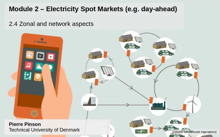
Prices may vary geographically

Remember there is a network involved, and power has to flow... This was not accounted for so far!

2/19

Exchange capacity limitations

There is a maximum amount of energy that may be exchanged from

• ne location to the next

When this limit is reached, one talks about congestion and prices for connected areas will differ Exchange capacity limitations are directly related to network constraints and

• perational practice

3/19

Approaches to handling exchange capacity limitations

There are basically two philosophies, developed on both sides of the Atlantic Ocean, i.e., in Europe and the USA Europe US System Operator TSO ISO Market Operator

• Ind. Market Operator

ISO Offers Market products Unit capabilities Clearing Supply-demand equilibrium UCED problem Network representation Highly simplified Fairly detailed Prices Zonal Nodal TSO: Transmission System Operator ISO: Independent System Operator UCED: Unit Commitment and Economic Dispatch

4/19

Illustration of zonal and nodal pricing

Scandinavia (Zonal):

Go visit: http://nordpoolgroup.com

Midwest US (Nodal): Go visit: https://www.misoenergy.org

5/19

From system price to area prices

Let us revisit our previous market clearing example,

considering two areas DTU-West and DTU-East, and with a transmission capacity of 40 MW (so, only 40MWh can flow)

6/19

Localization of offers

Demand: (for a total of 1065 MWh) Company id Amount (MWh) Price (e/MWh) Area CleanRetail D1 250 200 DTU-West El4You D2 300 110 DTU-East EVcharge D3 120 100 DTU-West QualiWatt D4 80 90 DTU-East IntelliWatt D5 40 85 DTU-West El4You D6 70 75 DTU-West CleanRetail D7 60 65 DTU-East IntelliWatt D8 45 40 DTU-West QualiWatt D9 30 38 DTU-West IntelliWatt D10 35 31 DTU-East CleanRetail D11 25 24 DTU-East El4You D12 10 16 DTU-East

7/19

And on the supply side

Supply: (for a total of 1435 MWh) Company id Amount (MWh) Price (e/MWh) Area RT R

• G1

120 DTU-West WeTrustInWind G2 50 DTU-East BlueHydro G3 200 15 DTU-West RT R

• G4

400 30 DTU-East KøbenhavnCHP G5 60 32.5 DTU-West KøbenhavnCHP G6 50 34 DTU-East KøbenhavnCHP G7 60 36 DTU-West DirtyPower G8 100 37.5 DTU-West DirtyPower G9 70 39 DTU-West DirtyPower G10 50 40 DTU-West RT R

• G11

70 60 DTU-East RT R

• G12

45 70 DTU-West SafePeak G13 50 100 DTU-East SafePeak G14 60 150 DTU-East SafePeak G15 50 200 DTU-East

8/19

Localizing the previous market-clearing results

Following previous market clearing results, one obtains

Supply side: {G1, G3, G5, G7, G8} (but only 55 MWh for G8) - Total: 495 MWh Demand side: {D1, D3, D5, D6, D8, D9} - Total: 555 MWh → Deficit of 60 MWh Supply side: {G2, G4, G6} - Total: 500 MWh Demand side: {D2, D4, D7} - Total: 440 MWh → Surplus of 60 MWh

BUT, only 40 MWh can flow through the interconnection!

9/19

Intuition based on an import-export approach

Due to transmission constraints, the market has to split and becomes two markets

→

DTU-West

quantity [MWh] price [Euros/MWh] 500 50 100 150 200

DTU-East

quantity [MWh] price [Euros/MWh] 500 50 100 150 200

In practice:

2 market zones with their own supply-demand equilibrium extra (price-independent) consumption/generation offers representing the transmission from one zone to the next to be added

10/19

Adding transmission-related offers

Extra supply in the high price area, i.e., DTU-West (40 MWh coming from DTU-East)

quantity [MWh] price [Euros/MWh]

• 500

50 100 150 200

Extra consumption in the low price area, i.e., DTU-East (40 MWh for DTU-West)

quantity [MWh] price [Euros/MWh]

• 500

50 100 150 200

Power ought to flow from the low price area to the high price area

11/19

Market clearing results for both zones

The same type of LP problems as introduced before is solved

for each zone individually, with the extra consumption/generation offers representing the amount of energy transmitted Supply side: {G1, G3, G5, G7, G8} (but only 75 MWh for G8) - Total: 515 MWh Demand side: {D1, D3, D5, D6, D8, D9} - Total: 555 MWh → Zonal price: 37.5 e Supply side: {G2, G4, G6} (but only 30 MWh for G6) - Total: 480 MWh Demand side: {D2, D4, D7} - Total: 440 MWh → Zonal price: 34 e

12/19

More elegantly with flow-based coupling

Instead of boldly splitting the market, one could instead acknowledge how power flows... This allows clearing a single market with geographically differentiated prices

• ur DTU system with 2 zones

can be modelled as a 2-bus system, loads and generators are associated to the relevant bus DC power flow is assumed as commonly done at transmission level

13/19

Formulating the market clearing

The network-constrained social welfare maximization problem can be written as: max

{y D

i },{y G i }

• i

λD

i y D i −

• j

λG

j y G j

subject to

• i

y D,West

i

−

• j

y G,West

j

= B∆δ

• i

y D,East

i

−

• j

y G,East

j

= −B∆δ 0 ≤ y D

i

≤ PD

i , i = 1, . . . , ND

0 ≤ y G

j

≤ PG

j , j = 1, . . . , NG

− 40 ≤ B∆δ ≤ 40 where:

B is the absolute value of susceptance (physical constant) of the interconnection between DTU-West and DTU-East ∆δ is the difference of voltage angles between the 2 buses → B∆δ represents the signed power flow from DTU-West to DTU-East

14/19

Obtaining the zonal prices

As for the case of a single zone, the dual LP allows obtaining market-clearing prices These 2 prices corresponds to the Lagrange multipliers for the 2 equality constraints (i.e., balance equations): max

{y D

i },{y G i }

• i

λD

i y D i −

• j

λG

j y G j

subject to

• i

y D,West

i

−

• j

y G,West

j

= B∆δ : λS,West

• i

y D,East

i

−

• j

y G,East

j

= −B∆δ : λS,East 0 ≤ y D

i

≤ PD

i , i = 1, . . . , ND

0 ≤ y G

j

≤ PG

j , j = 1, . . . , NG

− 40 ≤ B∆δ ≤ 40

15/19

Results for our auction example

Results are the same than those based on the import-export approach

Supply side: {G1, G3, G5, G7, G8} (but only 75 MWh for G8) - Total: 515 MWh Demand side: {D1, D3, D5, D6, D8, D9} - Total: 555 MWh → Zonal price: 37.5 e Supply side: {G2, G4, G6} (but only 30 MWh for G6) - Total: 480 MWh Demand side: {D2, D4, D7} - Total: 440 MWh → Zonal price: 34 e

However, all zones are modeled at once, and the approach can scale readily

16/19

Final extension to nodal pricing

In a US-like setup, each node of the power system is to be seen as an area For a system with K nodes, the network-constrained social welfare maximization market-clearing writes: max

{y D

i },{y G i }

• i

λD

i y D i −

• j

λG

j y G j

subject to

• i

y D,k

i

−

• j

y G,k

j

=

• l∈Lk

Bkl(δk − δl), k = 1, . . . , K : λS,k 0 ≤ y D

i

≤ PD

i , i = 1, . . . , ND

0 ≤ y G

j

≤ PG

j , j = 1, . . . , NG

− Ckl ≤ Bkl(δk − δl) ≤ Ckl , k, l ∈ LN where

LN is the set of nodes, Lk the set of nodes connected to node k Bkl are the line suseptances, (δk − δl) the phase angle differences λS,k are the K nodal prices

[Extra: Enerdynamics (2012). Locational Marginal Pricing. Electricity Markets Dynamics online course (video)] 17/19

Settlement under zonal and nodal pricing

Market participants are subject to the price where they are physically located, i.e.,

Consumption side: RDA,D

i

= −λS,locationy D

i , RDA,D i

≤ 0, (since being a payment) Supply side: RDA,G

j

= λS,locationy G

j , RDA,G j

≥ 0 (since being a revenue)

Payment and revenues for our example market clearing

Consumption side (payments): D1 pays 250 × 37.5 = 9375 e, (RDA,D

9

= −9375) D2 pays 300 × 34 = 10200 e, (RDA,D

9

= −10200), etc. D9 pays 30 × 37.5 = 1125 e, (RDA,D

9

= −1125) Supply side (revenues): G1 receives 120 × 37.5 = 4500 e, (RDA,G

8

= 4500) G2 receives 50 × 34 = 1700 e, (RDA,G

2

= 1700), etc. G8 receives 55 × 37.5 = 2062.5 e, (RDA,G

8

= 2062.5)

18/19

Settlement under zonal and nodal pricing

Market participants are subject to the price where they are physically located, i.e.,

Consumption side: RDA,D

i

= −λS,locationy D

i , RDA,D i

≤ 0, (since being a payment) Supply side: RDA,G

j

= λS,locationy G

j , RDA,G j

≥ 0 (since being a revenue)

Payment and revenues for our example market clearing

Consumption side (payments): D1 pays 250 × 37.5 = 9375 e, (RDA,D

9

= −9375) D2 pays 300 × 34 = 10200 e, (RDA,D

9

= −10200), etc. D9 pays 30 × 37.5 = 1125 e, (RDA,D

9

= −1125) Supply side (revenues): G1 receives 120 × 37.5 = 4500 e, (RDA,G

8

= 4500) G2 receives 50 × 34 = 1700 e, (RDA,G

2

= 1700), etc. G8 receives 55 × 37.5 = 2062.5 e, (RDA,G

8

= 2062.5)

The market is not budget balanced anymore, since the sum of consumer payments is greater that the sum of supplier revenues The difference defines a congestion rent to be collected by the system operator(s)

18/19