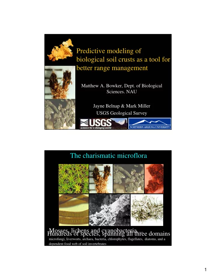
Predictive modeling of biological soil crusts as a tool for better - PDF document

Predictive modeling of biological soil crusts as a tool for better range management Matthew A. Bowker, Dept. of Biological Sciences. NAU Jayne Belnap & Mark Miller USGS Geological Survey The charismatic microflora Mosses, lichens and cyanobacteria… Hundreds of species, spanning all three domains microfungi, liverworts, archaea, bacteria, chlorophytes, flagellates, diatoms, and a dependent food web of soil invertebrates 1

BSCs harbor ecosystem engineers Organisms that control the availability of resources and living space for other organisms by causing physical state changes in biotic or abiotic materials (Jones et al. 1994, 1998) Microcoleus 1) Surface stabilization (increased living space) 2) Hydrology effects (increased water availability) 3) Dust trapping (increased nutrient availability) Image: J. Johansen Ecosystem engineering: soil stabilization cyanobacteria sheath w/clay Sand grains cyanobacteria Chemically Physically EROSION Hu et. al 2002 Mazor et. al 1996 Belnap & Gardner 1993 2

Ecosystem engineering: soil stabilization 40 Soil stability (slake test 2 ) 35 30 25 20 15 10 R 2 Rsqr = 0.90 5 0 0.000 0.002 0.004 0.006 0.008 0.010 0.012 0.014 0.016 0.018 0.020 Cyanobacterial biomass (chl a mg g soil-1 ) Bowker, Miller & Belnap unpublished Ecosystem engineering: hydrology effects Runoff Infiltration Runoff Infiltration smooth bumpy crusts (hot) crusts (cold) Issa et al. 1999 both types retain water longer- surface sealing (e.g. Alexander & Calvo 1992, George et al. 2003) 3

Ecosystem engineering: dust trapping Reynolds et al. 2001 Surfaces with BSCs enriched in eolian dust Microcoleus Syntrichia compared to bedrock P: 2 X K: 1.2 X Mg: 4.4 X Fe: 1.6 X Cu: 1.4 X Mn: 2.1 X Image: B. Mishler, Image: J. Johansen, Mo: 5 X Jepson Herbarium JCU BSC contributions to ecosystem function ~ equal to a continuous Photosynthesizers: leaf covering the ground mosses, lichens, cyanobacteria surface- Otto Lange C N Collema spp. Nostoc & Scytonema spp. 4

BSC contributions to ecosystem function: N- fixation How much N? (reviewed in Evans & Lange 2001) 7 - 18 kg ha -1 y -1 Sonoran desert: Kg ha -1 yr -1 10 – 100 kg ha -1 y -1 Great Basin: 0 1 – 4 kg ha -1 y -1 Colorado Plateau: 0.4 1 kg ha -1 y -1 Australia: 1.5 2.1 3 – 9 kg ha -1 y -1 Nigeria: 2.8 up to 10 kg ha -1 PER DAY! High Arctic: 3.5 5.2 130 km Bowker, Miller & Belnap unpublished Because… + Ecosystem engineering + Ecosystem functioning & services And…management seeks to maintain, preserve and restore ecosystem processes Management must incorporate BSCs in decision making 5

Worldwide crusts are in decline due to… Livestock Agriculture Urbanization Climate change Desertification is widespread in the US = desertification Symptoms: erosion, of rangelands decreased productivity, $23 billion y -1 soil fertility loss, decreased ecosystem services (Dregne & Chou 1992) Rangeland health (Pellant et al. 2000) Site/soil Hydrologic Biotic stability Function integrity 17 indicators CRUSTS Degree of departure from reference 6

~2 million acres of complexity! 130 km The Mission: establish reference conditions Map outputs Inputs Potential crust Crust data condition (base) Statistical model: cover, biomass, potential soil diversity crust Crust function & Env. data properties (interpretive) elevation, precipitation, soils 7

Input data Potential crust Crust data condition (base) Statistical model: potential soil crust Crust function & Env. data properties (interpretive) Stratified field sampling: soil X precipitation NRCS soil map Field 200+ map units 9 map units surveys (including rock-dominated) sampled relatively 111 sites undisturbed sites 8

Soil types: eight types + rock dominated Precipitation gradient silty to sandy clay bentonitic sandy silty non-bent. silty shale limestone gypsiferous +CaCO 3 -CaCO 3 kaiparowits calcareous non-calc. siliceous Publicly available climate data Digital elevation models Average annual precipitation USGS PRISM 9

Modeling Potential crust Crust data condition (base) Statistical model: potential soil crust Crust function & Env. data properties (interpretive) CART (tree) model Response: moss cover in limestone calcareous soil non-bentonitic gypsiferous Predictors: soil non-calcareous bentonitic siliceous kaiparowits precipitation elevation elevation soil soil precip. non-bent low limestone non-calc 25.4 ± 11.1 15.0 ± 9.2 1.8 ± 2.4 calc, gyps, siliceous bent or kaip high 3.5 ± 2.4 bent or kaip high & dry high & wet 7.1 ± 4.2 12.2 ± 2.7 calc or gyps calc or gyps 10

Determining how good the models are: model performance Total Lichen Cover 1) Randomly withheld 12% 0.4 of data R 2 Model 0.3 lichen 0.69 Observed 0.2 2) Generate model moss 0.55 0.1 R 2 = 0.69 dark cyano 0.49 0 3) Test model against withheld 0 0.1 0.2 0.3 0.4 0.5 0.6 light cyano 0.22 Predicted data using linear regression chl. a 0.09 spp. richness 0.60 4) Repeat 5 times (bootstrapping) Outputs: “base” maps Potential crust condition (base) Crust data Statistical model: potential soil crust Env. data Crust function & properties (interpretive) 11

An example base map for total moss cover Total moss cover Two more base models Total lichen Dark cyanobacterial crust very different! 12

Different cover types can be summed R 2 = 0.64 Moss + lichen + dark cyano cover Using the models 1) Collect crust cover and ground cover data for sites to be evaluated e.g. point intercept transect crust functional groups or total crust cover 2) Compute cover data as percent of available habitat 40% cover 80% cover Pics here 50% available habitat 95% available habitat 80/95 = 84% cover of avail. habitat 40/50 = 80% cover of avail. habitat 3) Determine potential by locating your site on my maps 13

An example using the rangeland health dataset We selected 4 sites because they had varying potential crust cover formatting data for comparison with mine: Site ID litter rock plant bare crust all crust % avail. habitat E0002 12 0 38 36 14 20 21 E0091 4 0 33 63 0 0 0 E0134 26 4 28 36 2 2 3 E1502 14 24 50 10 2 5 8 14

4% 21% 0% 58% Assessing departure from potential 100 100 Percent cover 0 0 E0134 E0091 E0002 E1502 15

Limitations and caveats: assumes crusts are static Crust cover changes, even in the absence of disturbance My maps are a conservative estimate of potential crust cover because they are based on drought years Limitations and caveats: based upon minimal slope-aspect effect I primarily sampled flat sites N more cover less cover model OK model OK 16

Limitations and caveats: assumes soil map units are homogenous NRCS maps “map unit complexes” 5001- Mido fine sand 2-15% slopes Mido fine sand 85% Dune land 5% Mido family & similar 5% Earlweed & similar 5% = Calcareous sand Limitations and caveats: assumes soil map units are homogenous If you think your site deviates from my maps, you can classify it yourself* and use the trees d) Total light cyanobacterial crust R 2 = 0.80 soil L,G,NC,S,B C,NB,K elevation elevation # # 1668 > 1668 1505 > 1505 soil elevation L,G,NC S,B # 1632 > 1632 44.6% 48.2% ppt . # 20 > 20 68.1% 51.2% 36.1% 35.9% 11.6% * I owe you decision rules to classify soils 17

Outputs: interpretive maps Potential crust condition (base) Crust data Statistical model: potential soil crust Env. data Crust function & properties (interpretive) Base model of species richness Gypsiferous takes the prize # species 0 0.3 5.6 9.2 12.3 R 2 = 0.60 15.1 18.4 20.3 130 km 18

An interpretive model: N fixation base models + published rates (Belnap 2001) Kg ha -1 yr -1 0 0.4 1.5 2.1 2.8 3.5 5.2 130 km Identification of conservation priorities Spp. richness + N-fix (equal weight) Other input options: C-fixation Eolian dust retention Surface roughness Endemic/rare species Surface stabilization Weighting is 130 km user-defined = highest priorities 19

Conclusions Rangeland health + assessment + GSENM crust models Setting appropriate Better restoration goals Expanded crust models informed + for Colorado Plateau Estimating ecosystem land services management + ID of conservation priorities Thanks! • Planning/Insight/Critique: Kent Sutcliffe and NRCS staff, Roger Rosentreter, Thom O’Dell, Nancy Johnson, Johnson & Sisk labs (NAU) • Logistics, site suggestions: John Spence, Tim Graham, Harry Barber, Sean Stewart, Joel Tuhey, Angie Evenden, Paul Evangelista, Paul Chapman, and the GSENM staff • Field/Lab Assistance: Kate Kurtz, Chris Nelms, Sasha Reed, Bernadette Graham, Moab lab folks, Jenn Brundage, Laura Pfenninger, Sara Bartlett, Laura & Walt Fertig, Elaine Kneller Kneller • Modeling advice: John Prather, Walt Fertig • Funding: BLM, Merriam-Powell Center for Environmental Research And soil crusts everywhere!!!! 20