Model Predictive Control Model Predictive Control of Hybrid Systems - - PowerPoint PPT Presentation

Model Predictive Control Model Predictive Control

• f Hybrid Systems
• f Hybrid Systems

Alberto Bemporad Alberto Bemporad

• Dip. di
• Dip. di Ingegneria

Ingegneria dell’Informazione dell’Informazione Università Università degli degli Studi Studi di Siena di Siena

Università degli Studi di Siena Facoltà di Ingegneria

bemporad@dii.unisi.it bemporad@dii.unisi.it http:// http://www.dii.unisi.it/~bemporad www.dii.unisi.it/~bemporad

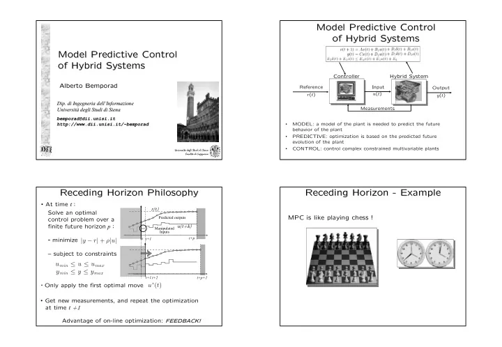
Model Predictive Control Model Predictive Control

• f Hybrid Systems
• f Hybrid Systems

y(t) u(t)

Hybrid System

Reference r(t) Output Input Measurements

Controller

• MODEL: a model of the plant is needed to predict the future

behavior of the plant

• PREDICTIVE: optimization is based on the predicted future

evolution of the plant

• CONTROL: control complex constrained multivariable plants

Receding Horizon Philosophy Receding Horizon Philosophy

• Only apply the first optimal move

Solve an optimal control problem over a finite future horizon p : – minimize – subject to constraints

Predicted outputs Manipulated Inputs t t+1 t+p

u(t+k) r(t)

t+1 t+2 t+p+1

• At time t :
• Get new measurements, and repeat the optimization

at time t +1 Advantage of on-line optimization: FEED

FEEDBAC BACK!

|y à r| + ú|u| umin ô u ô umax ymin ô y ô ymax uã(t)

Receding Horizon Receding Horizon -

• Example

Example

MPC is like playing chess !

• Apply only (discard the remaining optimal inputs)
• At time t

solve with respect to the finite-horizon open-loop, optimal control problem:

u(t) =uã(t)

MPC for Hybrid Systems MPC for Hybrid Systems

Predicted

• utputs

Manipulated y(t+k|t) Inputs t t+1 t+T future past u(t+k)

• Repeat the whole optimization at time t+1

Model Predictive (MPC) Control

Closed Closed-

• Loop Stability

Loop Stability

Proof: Easily follows from standard Lyapunov arguments

(Bemporad, Morari 1999)

Stability Proof Stability Proof

Note: Glob Global opt

• ptimum not

imum not ne needed for convergence ! eded for convergence ! Lyapunov function

x(t + 1) = 0.8 cosë(t) à sinë(t) sinë(t) cosë(t) " # x(t) + 1 ô õ u(t) y(t) = 0 1 [ ] x(t) ë(t) = 3 ù if [1 0]x(t) õ 0 à 3 ù if [1 0]x(t) < 0     

Open loop: Switching System:

Hybrid MPC Hybrid MPC -

• Example

Example

Closed loop:

y(t), r(t) u(t)

time t time t

Constraint: à 1 ô u(t) ô 1

Optimal Control of Hybrid Systems: Optimal Control of Hybrid Systems: Computational Aspects Computational Aspects

Mixed Integer Quadratic Program (MIQP)

MIQP Formulation of MPC MIQP Formulation of MPC

(Bemporad, Morari, 1999)

MILP MILP Formulation of MPC Formulation of MPC

(Bemporad, Borrelli, Morari, 2000)

min

ø

J(ø, x(t)) = X

k=0 Tà1

ïx

i + ïu i

s.t.Gø ô W + Sx(t) Mixed Integer Linear Program (MILP)

• Set ø,[ïx

1, . . ., ïx Ny, ïu 1, . . ., ïTà1, U, î, z]

• Introduce slack variables:

ïx

k

õ [Qy(t + k|t)]i i = 1, . . ., p, k = 1, . . ., T à 1 ïx

k

õ à [Qy(t + k|t)]i i = 1, . . ., p, k = 1, . . ., T à 1 ïu

k

õ [Ru(t + k))]i i = 1, . . ., m, k = 0, . . ., T à 1 ïu

k

õ à [Ru(t + k))]i i = 1, . . ., m, k = 0, . . ., T à 1

ïx

k

õ kQy(t + k|t)k∞ ïu

k

õ kRu(t + k)k∞

min |x| min ï s.t. ï õ x ï õ à x

• General purpose Branch & Bound/Branch & Cut solvers available

for MILP and MIQP (CPLEX, Xpress-MP, BARON, GLPK, ...)

BUT

• Mixed-Integer Programming is NP-hard

Mixed Mixed-

• Integer Program Solvers

Integer Program Solvers

Phase transitions have been found in computationally hard problems.

(Monasson et al., Nature, 1999)

• No need to reach global optimum (see proof of the theorem),

although performance deteriorates

http://plato.la.asu.edu/bench.html

More solvers and benchmarks:

0 2

3 2 3 4 5 4 5

Ratio of Constraints to Variables

6 7 6 7 8 1000 1000 3000 3000

Cost of Computation

2000 2000 4000 4000

50 var 40 var 20 var

… but not for fast sampling (e.g. 10 ms) / cheap hardware ! Good for large sampling times (e.g., 1 h) / expensive hardware …

Explicit Form of Explicit Form of Model Predictive Control Model Predictive Control via via Multiparametric Multiparametric Programming Programming On On-

• Line vs. Off

Line vs. Off-

• Line Optimization

Line Optimization

• On-line optimization: given x(t), solve the problem at each time step t

multi-parametric Mixed Integer Linear Program (mp-MILP) Mixed-Integer Linear Program (MILP)

• Off-line optimization: solve the MILP fo

for a r all x(t)

minUJ(U, x(t)), P

k=0 Tà1

kQy(t + k + 1|t)k∞ + kRu(t + k)k∞

• subj. to

MLD model x(t|t) = x(t) x(t + T|t) = 0    min

ø

J(ø, x(t)),f 0ø s.t.Gø ô W + Fx(t)

• 6
• 4
• 2

20 40 60

• 6
• 4
• 2

20 40 60

CR{2,3} CR{1,4} CR{1,2,3} CR{1,3} x1 x2

Example of Example of Multiparametric Multiparametric Solution Solution

Multiparametric LP ( ) ø ∈ R2

• Linear Model:

Linear MPC Linear MPC

• Optimal control problem (quadratic performance index):
• Constraints:

• Substitution:

Linear MPC Linear MPC

Convex vex Q QUADR ADRATIC TIC PRO PROGRA RAM M (QP) P) (quadratic) (linear)

• Optimization problem:

Multiparametric Multiparametric Quadratic Programming Quadratic Programming

• Objective: solve the QP for

for a all

(Bemporad et al., 2002)

• Assumption:

(always satisfied if QP problem originates from

• ptimal control problem)

Linearity of the Solution Linearity of the Solution

From (1) :

In some neighborhood of x0, λ and U are explicit affine functions of x !

solve QP to find identify active constraints at KKT

• ptimality

conditions: From (2) : form matrices by collecting active constraints x0∈ X

Determining a Critical Region Determining a Critical Region

• Impose primal and dual feasibility:
• Remove redundant constraints

critical region CR0 CR0 = {Ax ô B} CR0

x-space x0

• X
• is the set of all and only parameters x for which

is the optimal combination of active constraints at the optimizer

G à , W à , S à CR0

linear inequalities in x !

Multiparametric Multiparametric QP QP

CR0 = {Ax ô B} Ri = {x ∈ X : Aix > Bi, Ajz ô Bj, ∀j < i}

The Theore rem: is a partition of

{CR0, R1, . . ., RN} X ò Rn

CR0

x-space x0

• R1

R2 RN R3 X R4

Proceed iteratively: for each region repeat the whole procedure with X ←Ri

Ri The recursive algorithm terminates after a finite number of steps, because the number of combinations

• f active constraints is finite

Multiparametric Multiparametric QP QP

CR0 = {Ax ô B} Ri = {x ∈ X : Aix > Bi, Ajz ô Bj, ∀j < i}

The Theore rem: is a partition of

{CR0, R1, . . ., RN} X ò Rn

CR0

x-space x0

• R1

R2 RN R3 X R4

Keep track of the CR already explored, don’t split CRs Note: while is characterizing a set of active constraints, is not Ri CR0 The active set of a neighboring region is found by using the active set of the current region + knowledge of the type of hyperplane we are crossing:

⇒ The corresponding constraint is adde dded to the active set ⇒ The corresponding constraint is withdr hdrawn from the active set

CR CR CR x1 x2 x1 x2 x1 x2

Mp Mp-

• QP

QP – – More efficient method More efficient method

(Tøndel, Johansen, Bemporad, 2003)

Mp Mp-

• QP

QP Properties Properties

continuous, piecewise affine convex, continuous, piecewise quadratic, C1 (if no degeneracy) Corol Corollary: The linear MPC controller is a continuous piecewise affine function of the state

Complexity Reduction Complexity Reduction

Regions where the first component of the solution is the same can be joined (when their union is convex). (Bemporad, Fukuda, Torrisi,

Computational Geometry, 2001)

• 2.5
• 2
• 1.5
• 1
• 0.5

0.5 1 1.5 2 2.5

• 2.5
• 2
• 1.5
• 1
• 0.5

0.5 1 1.5 2 2.5 CR1 CR2 CR3 CR4 CR5 CR6 CR7 CR8 CR9

• 2.5
• 2
• 1.5
• 1
• 0.5

0.5 1 1.5 2 2.5

• 2.5
• 2
• 1.5
• 1
• 0.5

0.5 1 1.5 2 2.5 CR1 CR2 CR3 CR4 CR5 CR6 CR7

Double Integrator Example Double Integrator Example

y(t) = s2

1 u(t)

x(t + 1) = 1 1 1 ô õ x(t) + 1 ô õ u(t) y(t) = 1 [ ] x(t)

• System:

à 1 ô u(t) ô 1

• Constraints:
• Control objective: minimize

P

t=0 ∞ y0(t)y(t) + 100 1 u2(t)

ut+k = KLQ x(t + k|t) ∀k õ Nu

• Optimization problem: for Nu=2

sampl mpling + Z ng + ZOH Ts=1 =1 s

(cost function is normalized by max λ(H))

mp mp-

• QP solution

QP solution

Nu=2

Complexity Complexity

Nu=3 Nu=4 Nu=5 Nu=6

5 10 15 20 20 40 CPU time 5 10 15 20 100 200 300 # Regions # free moves

Complexity Complexity

• Numerical Tests:
• Worst
• c

ase complexity analysis:

M,P

`=0 q ` q

( ) = 2q Nr ô P

k=0 Mà1 k!qk

combinations of active constraints upper

• b
• und to the number of regions

Computation time (s) [Matlab 5.3, Pentium II 300MHz] Number of regions in the state-space partition

Extensions Extensions

• Tracking of reference r(t) :
• Rejection of measured

disturbance v(t) :

• Soft constraints:
• Variable constraints:

îu(t) = F(x(t), u(t à 1), r(t)) îu(t) = F(x(t), u(t à 1), v(t)) u(t) = F(x(t), umin(t), . . ., ymax(t)) u(t) = F(x(t)) ymin à ï ô y(t + k|t) ô ymax + ï umin(t) ô u(t + k) ô umax(t) ymin(t) ô y(t + k|t) ô ymax(t)

• Linear norms:

minU J(U, x(t)),P

k=0 p

kQy(t + k|t)k∞ + kRu(t + k)k∞

(Bemporad, Borrelli, Morari, IEEE TAC, 2002)

Closed Closed-

• Loop MPC and Hybrid Systems

Loop MPC and Hybrid Systems

Motivation: Use hybrid techniques to analyze closed-loop MPC systems !

(Bemporad, Heemels, De Schutter IEEE TAC, 2002)

DHA DHA

MPC Regulation of a Ball on a Plate MPC Regulation of a Ball on a Plate

• Tune an MPC

controller by simulation, using the MPC Sim C Simulink link Toolb Toolbox

• Get the explic

explicit it solutio solution of the MPC controller.

• Validate the controller
• n exp

experimen ents ts.

Ta Task sk:

Ball&Plate Experiment Ball&Plate Experiment

• Specifications:

Angle:

• 17 deg … +17deg

Plate:

• 30 cm …+30 cm

Input Voltage: -10 V… +10 V Computer: PENTIUM166 Sampling Time:30 ms

• Model:

LTI 14 states Constraints on inputs and states

y α β x

α' β' δ γ

E.g: MPC Toolbox for Matlab

• Step 1: Tune the MPC controller (in simulation)

General Philosophy: (1) MPC Design General Philosophy: (1) MPC Design

(Bemporad, Morari, Ricker, 2003)

General Philosophy: (2) Implementation General Philosophy: (2) Implementation

• Step 2: Solve mp
• Q

P and implement Explicit MPC E.g: Real

• T

ime Workshop + xPC Toolbox

MPC Tuning MPC Tuning

Sampling time:

Ts = 30 30 ms ms p = 50 50 m = 2

m p u

1 (hard constraint) 5

y Prediction horizon: Free control moves: Output constraint horizon: Input constraint horizon: Weight on position error: Weight on input voltage changes:

1 (soft constraint) 1

Explicit MPC Solution Explicit MPC Solution

x-M

• MPC: sections at αx=0, αx=0, ux=0, rx=18, rα=0

Region 1: Region 1: Region 6: Region 6: Region 16: Region 16:

Saturation at -10 Saturation at +10 LQR Controller (near Equilibrium)

6 1 16 16 6 16 16

1

• x: 22 Regions, y: 23 Regions

Con Controll ller:

MPC Regulation of a Ball on a Plate MPC Regulation of a Ball on a Plate

• Tune an MPC

controller by simulation, using the MP MPC S Simulink Toolb Toolbox .

• Get the explic

explicit it solutio solution of the MPC controller. Validate the controller on ex expe perime ment nts.

Desi sign S gn Steps: eps:

Comments on Explicit MPC Comments on Explicit MPC

• Multiparametric Quadratic Programs (mp-QP) can be solved efficiently
• Explicit solution of MPC controlleru = f(x) is Piecewise Affine

Elimina nate he te heavy on- vy on-line computa e computation for

• n for MPC

Ma Make M MPC sui suitable for for fa fast st/sma /small/chea /cheap pr processes

• cesses
• Model Predictive Control (MPC) can be solved off-line via mp-QP

MILP MILP Formulation of MPC Formulation of MPC

(Bemporad, Borrelli, Morari, 2000)

min

ø

J(ø, x(t)) = X

k=0 Tà1

ïx

i + ïu i

s.t.Gø ô W + Sx(t) Mixed Integer Linear Program (MILP)

• Set ø,[ïx

1, . . ., ïx Ny, ïu 1, . . ., ïTà1, U, î, z]

• Introduce slack variables:

ïx

k

õ [Qy(t + k|t)]i i = 1, . .., p, k = 1, . . ., T à 1 ïx

k

õ à [Qy(t + k|t)]i i = 1, . .., p, k = 1, . . ., T à 1 ïu

k

õ [Ru(t + k))]i i = 1, . . ., m, k = 0, . . ., T à 1 ïu

k

õ à [Ru(t + k))]i i = 1, . . ., m, k = 0, . . ., T à 1

ïx

k

õ kQy(t + k|t)k∞ ïu

k

õ kRu(t + k)k∞

min |x| min ï s.t. ï õ x ï õ à x

• Theorem

Theorem: The multiparametric solution is piecewise affine

s.t. Gøc + Eød ô W + Fx

min ø={øc,ød} f0øc + d0ød

(Dua, Pistikopoulos, 1999)

øc ∈ Rn ød ∈ {0, 1}m

• mp-MILP can be solved (by alternating MILPs and mp-LPs)

Multiparametric Multiparametric MILP MILP

• Corol
• rollary

ry: The MP The MPC control C controller i r is pi piecew ecewise af e affine ne in x

øã(x)

• Explicit solutions to finite
• t

ime optimal control problems for PWA systems can be obtained using a combination of

• Dynamic Programming
• Multiparametric Linear (1
• n
• rm, ∞
• n
• rm), or
• r Quadratic (squared 2
• n
• rm) programming

Solutions via Dynamic Programming Solutions via Dynamic Programming

(Borrelli, Bemporad, Baotic, Morari, 2003) (Mayne, ECC 2001)

Note: in the 2-norm case, the partition may not be polyhedral

Hybrid Control Example Hybrid Control Example (Revisited) (Revisited)

x(t + 1) = 0.8 cosë(t) à sinë(t) sinë(t) cosë(t) " # x(t) + 1 ô õ u(t) y(t) = 0 1 [ ]x(t) ë(t) = 3 ù if [1 0]x(t) õ 0 à 3 ù if [1 0]x(t) < 0     

Open loop: Closed loop: Switching System:

Hybrid Control Hybrid Control -

• Example

Example

y(t), r(t) u(t)

time t time t

Constraint: à 1 ô u(t) ô 1

• MLD system
• mp
• M

I LP optimization problem

to be solved in the region

• Computational complexity of mp
• M

I LP

min

v1

n oJ(v1

0, x(t)),P k=0 1

kQ1(v(k) à ue)k∞ + kQ2(î(k|t) àîe)k∞+ kQ3(z(k|t) àze)k∞ +kQ4(x(k|t) à xe)k∞ subject to constraints

à 5 ô x1 ô 5 à 5 ô x2 ô 5

Hybrid MPC Hybrid MPC -

• Example

Example

Linear constraints Continuous variables Binary variables Parameters Time to solve mp-MILP Number of regions 84 20 2 2 3 min 7

State x(t) 2 variables Input u(t) 1 variables

• Aux. binary vector δ(t)

1 variables

• Aux. continuous vector z(t)

4 variables

mp mp-

• MILP Solution

MILP Solution

PWA law law M MPC law law PWA law law M MPC law law

ñ

Prediction Horizon T=2

Linear constraints Continuous variables Binary variables Parameters Time to solve mp-MILP Number of regions 84 20 2 2 3 min 7

mp mp-

• MILP Solution

MILP Solution

Prediction Horizon T=3 Prediction Horizon T=4

X1 X2 X1 X2

Hybrid Control Example: Hybrid Control Example: Traction Control System Traction Control System

Control

• ntroller

suitable for real-time implementation

Improve driver’s ability to control a vehicle under adverse external conditions (wet or icy roads)

MLD hybrid framework + optimization-based control strategy

Vehicle Traction Control Vehicle Traction Control

Model

• del

nonlinear, uncertain, constraints

Simple Traction Model Simple Traction Model

• Tire torque τt is a function of

slip ∆ω and road surface adhesion coefficient µ

ω ç e = Je 1 üc à beωe à gr üt ò ó v çv = mvrt üt ∆ω = gr ωe à rt vv

• Mechanical system
• Manifold/fueling dynamics

üc = biüd(t à üf)

∆ω Wheel slip

Lateral Force Tire Forces Tire Slip Maximum Acceleration Longitudinal Force Slip Target Zone Maximum Cornering Maximum Braking Lateral Force Longitudinal Force Steer Angle

Tire Force Characteristics Tire Force Characteristics Hybrid Model Hybrid Model

Torque

Mixed-Logical Dynamical (MLD) Hybrid Model (discrete time)

Slip Torque µ

PWA Approximation

µ Slip

HY HYSDEL SDEL

(Hybrid S d Syste stems Desc scriptio ption L n Langua nguage ge)

Nonlinear tire torque τt =f(∆ω , µ)

(PWL Toolbox, Julian, 1999)

MLD Model MLD Model

State x(t) 9 variables Input u(t) 1 variable

• Aux. Binary

vars δ(t ) 3 variables

• Aux. Continuous vars z(t)

4 variables

The MLD matrices are automatically generated in Matlab format by HYSDEL

Performance and Constraints Performance and Constraints

minP

k=0 N

∆ω(k|t) à ∆ωdes | |

• Control objective:
• Constraints:
• Limits on the engine torque: à 20Nm ô üd ô 176Nm
• subj. to. MLD Dynamics
• Logic Constraint:
• Hysteresis

Experimental Apparatus Experimental Apparatus Experimental Apparatus Experimental Apparatus

Experiment Experiment

• >500 regions
• 20ms sampling time
• Pentium 266Mhz +

Labview

Hybrid Control Example: Hybrid Control Example: Cruise Control System Cruise Control System Hybrid Control Problem Hybrid Control Problem

Renault Clio 1.9 DTI RXE GOAL: command gear ratio, gas pedal, and brakes to trac ack k a desired speed and minimize consumption

Hybrid Model Hybrid Model

ω =

ks Rg(i)x

ç mx ¨ = Fe à Fb à ìx ç Fe =

ks Rg(i)M

• Vehicle dynamics
• Transmission kinematics

discretized with sampling time Ts = 0.5 s

= engine torque = engine speed = gear

ω M i

= vehicle speed

x ç

= brake force

Fb

= traction force

Fe

Hybrid Model Hybrid Model

1000 2000 3000 4000 60 80 100 120 140 160 180

C+

e (ω)

• Max engine torque

Piecewise-linearization:

(PWL Toolbox, Julián, 1999)

http://www.renault.fr

Cà

e (ω) = ë1 + ì1ω

• Min engine torque

requires: 4 binary aux variables 4 continuous aux variables

à Cà

e (ω) ô M ô C+ e (ω)

• Engine torque

Hybrid Model Hybrid Model

ω =

ks Rg(i)x

ç Fe =

ks Rg(i)M

• Gear selection (traction force):

Fe = FeR + Fe1 + Fe2 + Fe3 + Fe4 + Fe5

depends on gear #i define auxiliary continuous variables: similarly, also requires 6 auxiliary continuous variables

• Gear selection (engine/vehicle speed):
• Gear selection:

gi ∈ {0, 1}

for each gear #i, define a binary input

IF gi = 1 THEN Fei =

ks Rg(i)M ELSE 0

Hybrid Model Hybrid Model

• MLD model

x(t + 1) = Ax(t) + B1u(t) y(t) = Cx(t) + D1u(t) + B2î(t) + B3z(t) + D2î(t) + D3z(t) E2î(t) + E3z(t) ô E4x(t) + E1u(t) + E5

• 2 continuous states:
• 2 continuous inputs:
• 6 binary inputs:
• 1 continuous output:
• 4 auxiliary binary vars:
• 16 auxiliary continuous vars:

(engine torque, brake force) (vehicle speed) (gears)

v M, Fb gR, g1, g2, g3, g4, g5

(vehicle position and speed)

x, v

(6 traction force, 6 engine speed, 4 PWL max engine torque) (PWL max engine torque breakpoints)

• 96 mixed-integer inequalities

Hysdel Hysdel Model Model

http://control.ethz.ch/~hybrid/hysdel

Hybrid Controller Hybrid Controller

• Max-speed controller

maxut J(ut, x(t)),v(t + 1|t)

• subj. to

MLD model x(t|t) = x(t) ú MILP optimization problem

( is irrelevant)

x(t) v(t) x(t)

50 100 150 200 250

Linear constraints Continuous variables Binary variables Parameters Time to solve mp-MILP (Sun Ultra 10) Number o

• f re

regions 96 18 10 1 45 s 11 11

Hybrid Controller Hybrid Controller

• Max-speed controller

50 100 50 100 150 200 Velocity (km/h) 50 100 1000 2000 3000 4000 5000 6000 Engine speed (rpm) Time (s) 50 100 50 100 150 200 Engine Torque (Nm) Time (s) 50 100 1 2 3 4 5 Gear 50 100 10 20 30 40 50 60 Power (kW) Time (s) 50 100

• 1
• 0.5

0.5 1 Fraction of Max Torque (Nm) 50 100

• 1
• 0.5

0.5 1 Road Slope (deg) Time (s) 50 100

• 1
• 0.5

0.5 1 Brakes (Nm)

Hybrid Controller Hybrid Controller

• Tracking controller

minutJ(ut, x(t)),|v(t + 1|t) à vd(t)| + ú|ω|

• subj. to

MLD model x(t|t) = x(t) ú v(t) vd(t)

40 80 120 160 200 50 100 150 200 250

MILP optimization problem

Linear constraints Continuous variables Binary variables Parameters Time to solve mp-MILP (Sun Ultra 10) Number o

• f re

regions 98 19 10 2 27 m 49 49

Hybrid Controller Hybrid Controller

• Tracking controller

100 200 20 40 60 80 100 120 Velocity (km/h), Desired velocity (km/h) 100 200 1000 2000 3000 4000 5000 6000 Engine speed (rpm) Time (s) 100 200

• 200
• 100

100 200 Engine Torque (Nm) Time (s) 100 200 1 2 3 4 5 Gear 100 200

• 100
• 50

50 100 Power (kW) Time (s) 100 200

• 1
• 0.5

0.5 1 Fraction of Max Torque (Nm) 100 200

• 6
• 4
• 2

2 4 6 Road Slope (deg) Time (s) 100 200 2000 4000 6000 8000 10000 Brakes (Nm)

minutJ(ut, x(t)),|v(t + 1|t) à vd(t)| + ú|ω|

ú = 0.001

Hybrid Controller Hybrid Controller

• Smoother tracking controller

minutJ(ut, x(t)),|v(t + 1|t) à vd(t)| + ú|ω|

• subj. to

|v(t + 1|t) à v(t)| < Tsamax MLD model x(t|t) = x(t)    v(t) vd(t)

40 80 120 160 200 50 100 150 200 250

MILP optimization problem

Linear constraints Continuous variables Binary variables Parameters Time to solve mp-MILP (Sun Ultra 10) Number o

• f re

regions 100 19 10 2 28 m 54 54

Hybrid Controller Hybrid Controller

• Smoother tracking controller

100 200 20 40 60 80 100 120 Velocity (km/h), Desired velocity (km/h) 100 200 1000 2000 3000 4000 5000 6000 Engine speed (rpm) Time (s) 100 200

• 200
• 100

100 200 Engine Torque (Nm) Time (s) 100 200 1 2 3 4 5 Gear 100 200

• 100
• 50

50 100 Power (kW) Time (s) 100 200

• 1
• 0.5

0.5 1 Fraction of Max Torque (Nm) 100 200

• 6
• 4
• 2

2 4 6 Road Slope (deg) Time (s) 100 200 2000 4000 6000 8000 10000 Brakes (Nm)