Practical Modeling Overview Introduction Like most engineering, - PowerPoint PPT Presentation

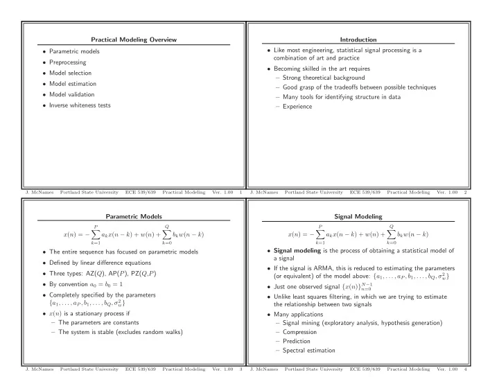
Practical Modeling Overview Introduction • Like most engineering, statistical signal processing is a • Parametric models combination of art and practice • Preprocessing • Becoming skilled in the art requires • Model selection – Strong theoretical background • Model estimation – Good grasp of the tradeoffs between possible techniques • Model validation – Many tools for identifying structure in data • Inverse whiteness tests – Experience J. McNames Portland State University ECE 539/639 Practical Modeling Ver. 1.00 1 J. McNames Portland State University ECE 539/639 Practical Modeling Ver. 1.00 2 Parametric Models Signal Modeling Q Q P P � � � � x ( n ) = − a k x ( n − k ) + w ( n ) + b k w ( n − k ) x ( n ) = − a k x ( n − k ) + w ( n ) + b k w ( n − k ) k =1 k =0 k =1 k =0 • Signal modeling is the process of obtaining a statistical model of • The entire sequence has focused on parametric models a signal • Defined by linear difference equations • If the signal is ARMA, this is reduced to estimating the parameters • Three types: AZ( Q ), AP( P ), PZ( Q , P ) (or equivalent) of the model above: { a 1 , . . . , a P , b 1 , . . . , b Q , σ 2 w } • By convention a 0 = b 0 = 1 • Just one observed signal { x ( n ) } N − 1 n =0 • Completely specified by the parameters • Unlike least squares filtering, in which we are trying to estimate { a 1 , . . . , a P , b 1 , . . . , b Q , σ 2 w } the relationship between two signals • x ( n ) is a stationary process if • Many applications – The parameters are constants – Signal mining (exploratory analysis, hypothesis generation) – The system is stable (excludes random walks) – Compression – Prediction – Spectral estimation J. McNames Portland State University ECE 539/639 Practical Modeling Ver. 1.00 3 J. McNames Portland State University ECE 539/639 Practical Modeling Ver. 1.00 4

Parametric Spectral Estimation Preprocessing • In practice some preprocessing is often necessary before the P Q � � x ( n ) = − a k x ( n − k ) + w ( n ) + b k w ( n − k ) techniques can be applied k =1 k =0 • Essentially slowly varying components must be eliminated 2 � � 1 + � Q k =1 b k e − jωk – DC components � � R x (e jω ) = σ 2 � � w 1 + � P � � – Linear or polynomial trends k =1 a k e − jωk � � – Seasonal variations • If we have a good estimate of the model parameters, we can plug them in to the PSD equation for ARMA processes – Unit poles (random walk effects) • If the parameters are close to the true values, we would expect the • Can often be achieved with highpass of difference filters PSD estimate to be accurate • If using a moving window, the window should span at least several • However, it is in no way an optimal estimate of the PSD periods of the lowest frequency component of interest • There are some methods that directly attempt to estimate the PSD in the frequency domain – Not discussed in this class • In practice, most people use plug-in estimates J. McNames Portland State University ECE 539/639 Practical Modeling Ver. 1.00 5 J. McNames Portland State University ECE 539/639 Practical Modeling Ver. 1.00 6 Model Building Process Model Selection • Goal is to select a parametric model to fit the data • Essentially three key steps 1. Model selection • Ideally would like the model to 2. Parameter estimation – Be as simple as possible 3. Validation – Fully explain the variation in the data – Have parameters that have physical meaning for the application • Good judgement and experience are necessary for all three – Be in a form that is mathematically tractable (e.g., linear in • Difficult (impossible?) to fully automate the parameters) • When possible, domain knowledge of the problem should guide this decision • In many instances, have to resort to data analysis methods J. McNames Portland State University ECE 539/639 Practical Modeling Ver. 1.00 7 J. McNames Portland State University ECE 539/639 Practical Modeling Ver. 1.00 8

Model Selection Through Data Analysis Parameter Estimation • Goal is to estimate the model parameters given the observed data • If considering only ARMA, AR, and MA processes can use the { x ( n ) } N − 1 autocorrelation and partial autocorrelation functions n =0 – MA processes have an autocorrelation of zero for ℓ > Q • Also called model fitting – AR processes have a partial autocorrelation of zero for ℓ > P • Many different approaches used in the literature – ARMA processes don’t have either – Least squares • Thus ACF and PACF are often used to select both – Maximum likelihood – Model structure: MA, AR, ARMA – Spectral matching (frequency domain estimation) – Model order: P and Q – Robust error measures – Moment matching • Keep in mind that a high order AR or MA process can serve as a good model of other types of processes – Bayesean approaches • Filter structure (e.g., direct or lattice) is not critical at this stage • Book focuses on least squares • If model structure is AP, leads to a closed form solution J. McNames Portland State University ECE 539/639 Practical Modeling Ver. 1.00 9 J. McNames Portland State University ECE 539/639 Practical Modeling Ver. 1.00 10 Model Validation Model Validation Through Data Analysis • Goals are • If the model is accurate, the residual or prediction error signal – Determine whether the model sufficiently “agrees” with the should be indistinguishable from white noise observed data • We can test for various properties of a white noise process to help – Describes the true source of the data identify statistical “structure” – Solves the application problem at hand • There are many techniques for this • If not, the first two steps are repeated – Autocorrelation function should be an impulse – Partial autocorrelation function should be an impulse • Data analysis techniques can help determine how well the model fits the observed data – Periodogram should be flat – The performance criterion doesn’t decrease too fast as the model order is increased – Cross validation (rarely used in signal processing, not sure why) • Specifics are in the text J. McNames Portland State University ECE 539/639 Practical Modeling Ver. 1.00 11 J. McNames Portland State University ECE 539/639 Practical Modeling Ver. 1.00 12