
SLIDE 1
1
MDPs cont, Lecture 25
Nov 24 2008
Review
- Critical components of MDPs
– State space and action space; Transition model; Reward function
- Value iteration
U(S) th t d f i d – U(S): the expected sum of maximum rewards achievable starting at a particular state – Bellman equation: – Bellman iteration: – Optimal policy:
∑
+ =
'
) ' ( ) ' , , ( max ) ( ) (
s a
s U s a s T s R s U γ
∑
=
' * *
) ' ( ) ' , , ( max arg ) (
s a
s U s a s T s π
∑
+ =
+ ' 1
) ' ( ) ' , , ( max ) ( ) (
s i a i
s U s a s T s R s U γ
Review: Policy Iteration
- Start with a randomly chosen initial policy π0
- Iterate until no change in utilities:
- 1. Policy evaluation: given a policy πi, calculate
the utility Ui(s) of every state s using policy πi by solving the system of equations:
- 2. Policy improvement: calculate the new policy
πi+1 using one‐step look‐ahead based on Ui(s):
∑
=
+ ' 1
) ' ( ) ' , , ( max arg ) (
s i a i
s U s a s T s π
Policy iteration comments
- Each step of policy iteration is guaranteed
to strictly improve the policy at some state when improvement is possible
- Converge to optimal policy
Converge to optimal policy
- Gives exact value of optimal policy
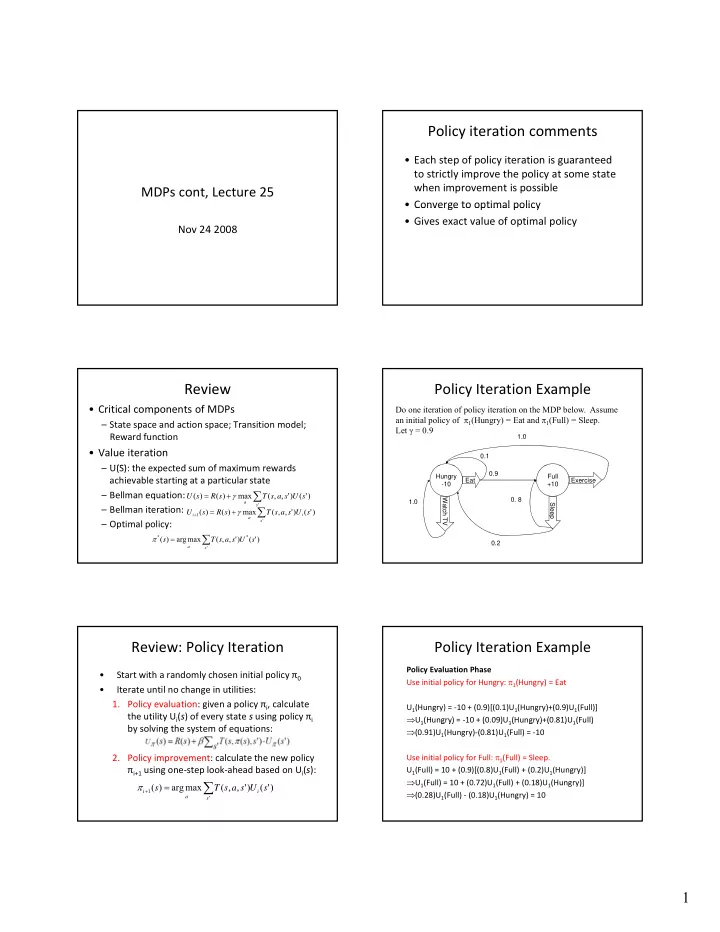
Policy Iteration Example
0.1 1.0
Do one iteration of policy iteration on the MDP below. Assume an initial policy of π1(Hungry) = Eat and π1(Full) = Sleep. Let γ = 0.9
Hungry
- 10
Full +10 Eat Exercise Watch TV Sleep 1.0 0.9
- 0. 8
0.2
Policy Iteration Example
Policy Evaluation Phase Use initial policy for Hungry: π1(Hungry) = Eat U1(Hungry) = ‐10 + (0.9)[(0.1)U1(Hungry)+(0.9)U1(Full)] ⇒U1(Hungry) = ‐10 + (0.09)U1(Hungry)+(0.81)U1(Full)
1(
g y) ( )
1(
g y) ( )
1(