[PPT] - Plug-and-Play Operation of Microgrids Florian D orfler ETH Z PowerPoint Presentation

SLIDE 1

Plug-and-Play Operation of Microgrids

Florian D¨

rfler

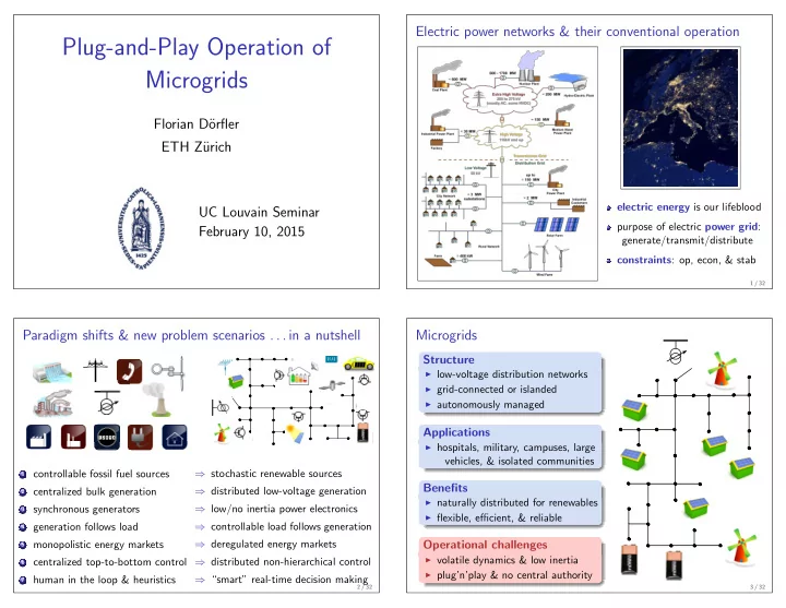
ETH Z¨ urich UC Louvain Seminar February 10, 2015 Electric power networks & their conventional operation

electric energy is our lifeblood purpose of electric power grid: generate/transmit/distribute constraints: op, econ, & stab

1 / 32

Paradigm shifts & new problem scenarios . . . in a nutshell

1 2 8 9 4

1 controllable fossil fuel sources 2 centralized bulk generation 3 synchronous generators 4 generation follows load 5 monopolistic energy markets 6 centralized top-to-bottom control 7 human in the loop & heuristics

⇒ stochastic renewable sources ⇒ distributed low-voltage generation ⇒ low/no inertia power electronics ⇒ controllable load follows generation ⇒ deregulated energy markets ⇒ distributed non-hierarchical control ⇒ “smart” real-time decision making

2 / 32

Microgrids

Structure

◮ low-voltage distribution networks ◮ grid-connected or islanded ◮ autonomously managed

Applications

◮ hospitals, military, campuses, large

vehicles, & isolated communities

Benefits

◮ naturally distributed for renewables ◮ flexible, efficient, & reliable

Operational challenges

◮ volatile dynamics & low inertia ◮ plug’n’play & no central authority

3 / 32

SLIDE 2

Conventional control architecture from bulk power ntwks

3. Tertiary control (offline)

Goal: optimize operation Strategy: centralized & forecast

2. Secondary control (slower)

Goal: maintain operating point Strategy: centralized

1. Primary control (fast)

Goal: stabilization & load sharing Strategy: decentralized

Microgrids: distributed, model-free,

nline & without time-scale separation

⇒ break vertical & horizontal hierarchy

4 / 32

A preview – plug-and-play operation architecture

flat hierarchy, distributed, no time-scale separations, & model-free . . .

source # 1

… … …

Power System

source # n source # 2

Secondary Control Tertiary Control Primary Control

Transceiver

Secondary Control Tertiary Control Primary Control

Transceiver

Secondary Control Tertiary Control Primary Control

Transceiver

5 / 32

Outline

Introduction Modeling Primary Control Tertiary Control Secondary Control Virtual Oscillator Control Conclusions

we will illustrate all theorems with experiments

modeling & assumptions

SLIDE 3

Modeling: a power system is a circuit

1 synchronous AC circuit with

harmonic waveforms Eiei(θi+ω∗t)

2 ZIP loads: constant impedance,

current, & power P∗

i + iQ∗ i

(today)

3 coupling via Kirchhoff & Ohm

Gij + i Bij i j

P ∗

i + i Q∗ i

I∗

i

Z∗

i

injection = power flows

4 identical lines G/B = const.

(equivalent to lossless case G/B = 0)

5 decoupling: Pi ≈ Pi(θ) & Qi ≈ Qi(E)

(near operating point)

◮ active power:

Pi =

j BijEiEj sin(θi − θj) + GijEiEj cos(θi − θj)

◮ reactive power:

Qi = −

j BijEiEj cos(θi − θj) + GijEiEj sin(θi − θj)

6 / 32

Modeling: a power system is a circuit

1 synchronous AC circuit with

harmonic waveforms Eiei(θi+ω∗t)

2 ZIP loads: constant impedance,

current, & power P∗

i + iQ∗ i

(today)

3 coupling via Kirchhoff & Ohm

Gij + i Bij i j

P ∗

i + i Q∗ i

I∗

i

Z∗

i

injection = power flows

4 identical lines G/B = const.

(equivalent to lossless case G/B = 0)

5 decoupling: Pi ≈ Pi(θ) & Qi ≈ Qi(E)

(near operating point)

◮ trigonometric active power flow:

Pi(θ) =

j Bij sin(θi − θj)

◮ polynomial reactive power flow:

Qi(E) = −

j BijEiEj (not today)

6 / 32

Modeling the “essential” network dynamics & controls

(models can be arbitrarily detailed)

1 synchronous machines (swing dynamics)

Mi ¨ θi = P∗

i + Pc i − Pi(θ)

2 DC & variable AC sources interfaced

with voltage-source converters P∗

i + Pc i = Pi(θ)

3 controllable loads (voltage-

and frequency-responsive) P∗

i + Pc i = Pi(θ)

mech. torque electr. torque

Eei(θ+ωt)

Pi(θ) , Qi(E)

Pi + i Qi

Eei(θ+ωt)

7 / 32

primary control (droop characteristic)

SLIDE 4

Decentralized primary control of active power

Emulate physics of dissipative coupled synchronous machines: Mi ¨ θ + Di ˙ θi = P∗

i −

j Bij sin(θi − θj)

Conventional wisdom: physics are naturally stable & sync frequency reveals power imbalance

P/ ˙ θ droop control:

(ωi − ω∗) ∝ (P∗

i − Pi(θ))

Di ˙

θi = P∗

i − Pi(θ)

Hz

power supplied power consumed 50 49 51 52 48

⇒ sum equations & set ˙ θi = ωsync: ωsync =

i P∗ i / i Di ωsync

8 / 32

Putting the pieces together...

differential-algebraic, nonlinear, large-scale closed loop

network physics

Di ˙ θi = (P ∗

i − Pi(θ))

droop control

power balance: P mech

i

= P ∗

i + P c i − Pi(θ)

power flow: Pi(θ) =

j Bij sin(θi − θj)

passive loads: 0 = P∗

i −

j Bij sin(θi − θj)

synchronous machines: Mi ¨ θi + Di ˙ θi = P∗

i −

j Bij sin(θi − θj)

inverter sources: Di ˙ θi = P∗

i −

j Bij sin(θi − θj)

controllable loads: Di ˙ θi = P∗

i −

j Bij sin(θi − θj)

9 / 32

A perspective from coupled oscillators

Mechanical oscillator network Angles (θ1, . . . , θn) evolve on Tn as Mi ¨ θi + Di ˙ θi = Ωi −

j Kij sin(θi − θj)

inertia constants Mi > 0
viscous damping Di > 0
external torques Ωi ∈ R
spring constants Kij ≥ 0

Droop-controlled power system 0 = P∗

i −

j Bij sin(θi − θj)

Di ˙ θi = P∗

i −

j Bij sin(θi − θj)

Mi ¨ θ + Di ˙ θi = P∗

i −

j Bij sin(θi − θj)

Ω1 Ω2 Ω3

P ∗

1

P ∗

2

P ∗

3

10 / 32

Closed-loop stability under droop control

Theorem: stability of droop control

[J. Simpson-Porco, FD, & F. Bullo, ’12]

∃ unique & exp. stable frequency sync ⇐ ⇒ active power flow is feasible Main proof ideas and some further results:

synchronization frequency:

ωsync = ω∗ +

sources P∗

i + loads P∗ i

sources Di

(∝ power balance)

steady-state power injections:

Pi = P∗

i

(load #i)

P∗

i − Di(ωsync−ω∗) (source #i)

(depend on Di & P∗

i )

stability via incremental Chetaev energy function [C. Zhao, E. Mallada, & FD ’14]

11 / 32

SLIDE 5

tertiary control (energy management)

Tertiary control and energy management

an offline resource allocation & scheduling problem

12 / 32

Tertiary control and energy management

an offline resource allocation & scheduling problem

minimize {cost of generation, losses, . . . } subject to equality constraints: power balance equations inequality constraints: flow/injection/voltage constraints logic constraints: commit generators yes/no . . .

12 / 32

Objective I: decentralized proportional load sharing

1) Sources have injection constraints: Pi(θ) ∈

0, Pi
2) Load must be serviceable:

0 ≤

loads P∗

j

≤

sources Pj

3) Fairness: load should be shared proportionally: Pi(θ) / Pi = Pj(θ) / Pj load

source # 2 source # 1

P1 P 1 P2 P 2

13 / 32

SLIDE 6

Objective I: decentralized proportional load sharing

1) Sources have injection constraints: Pi(θ) ∈

0, Pi
2) Load must be serviceable:

0 ≤

loads P∗

j

≤

sources Pj

3) Fairness: load should be shared proportionally: Pi(θ) / Pi = Pj(θ) / Pj A little calculation reveals in steady state: Pi(θ) Pi

!

= Pj(θ) Pj

⇒

P∗

i − (Diωsync − ω∗)

Pi

!

= P∗

j − (Djωsync − ω∗)

Pi . . . so choose P∗

i

Pi = P∗

j

Pj and Di Pi = Dj Pj

13 / 32

Objective I: decentralized proportional load sharing

1) Sources have injection constraints: Pi(θ) ∈

0, Pi
2) Load must be serviceable:

0 ≤

loads P∗

j

≤

sources Pj

3) Fairness: load should be shared proportionally: Pi(θ) / Pi = Pj(θ) / Pj

Theorem: fair proportional load sharing

[J. Simpson-Porco, FD, & F. Bullo, ’12]

Let the droop coefficients be selected proportionally: Di/Pi = Dj/Pj & P∗

i /Pi = P∗ j /Pj

The the following statements hold: (i) Proportional load sharing: Pi(θ) / Pi = Pj(θ) / Pj (ii) Constraints met: 0≤

loads P∗

j

≤

sources Pj ⇔ Pi(θ) ∈

0, Pi
13 / 32

Objective I: fair proportional load sharing

proportional load sharing is not always the right objective

load source # 2 source # 1 source # 3

14 / 32

Objective II: economic generation dispatch

minimize the total accumulated generation (many variations possible)

minimize θ∈Tn , u∈RnI f (u) =

sources αiu2

i

subject to source power balance: P∗

i + ui = Pi(θ)

load power balance: P∗

i = Pi(θ)

branch flow constraints: |θi − θj| ≤ γij < π/2 Unconstrained case: identical marginal costs αiu∗

i = αju∗ j

at optimality In conventional power system operation, the economic dispatch is solved offline, in a centralized way, & with a model & load forecast In a grid with distributed energy resources, the economic dispatch should be solved online, in a decentralized way, & without knowing a model

15 / 32

SLIDE 7

Objective II: decentralized dispatch optimization

Insight: droop-controlled system = decentralized primal/dual algorithm

Theorem: optimal droop

[FD, Simpson-Porco, & Bullo ’13, Zhao, Mallada, & FD ’14]

The following statements are equivalent: (i) the economic dispatch with cost coefficients αi is strictly feasible with global minimizer (θ∗, u∗). (ii) ∃ droop coefficients Di such that the power system possesses a unique & locally exp. stable sync’d solution θ. If (i) & (ii) are true, then θi ∼θ∗

i , u∗ i =−Di(ωsync−ω∗), & Diαi = Djαj .

recover load sharing for αi ∝ 1/Pi & similar results in constrained case similar results in transmission ntwks with DC flow [E. Mallada & S. Low, ’13]

& [N. Li, L. Chen, C. Zhao, & S. Low ’13] & [X. Zhang & A. Papachristodoulou, ’13] &

[M. Andreasson, D. V. Dimarogonas, K. H. Johansson, & H. Sandberg, ’13] & . . .

16 / 32

Some quick simulations & extensions

IEEE 39 New England with load step at 1s

2 4 6 8 10 0.01 0.02 0.03 0.04 0.05 0.06 0.07

Time (sec) Marginal cost (pu)

t → ∞: convergence to identical marginal costs

1 2 3 4 5 58.4 58.6 58.8 59 59.2 59.4 59.6 59.8 60 60.2 Time (sec) Frequency (Hz)

t → ∞: frequency ∝ power imbalance ⇒ strictly convex & differentiable cost f (u) =

sources ci(ui)

⇒ non-linear frequency droop curve c′

i −1( ˙

θi) = P∗

i − Pi(θ)

⇒ include dead-bands, saturation, etc.

Å Å ã ã

−1 −0.5 0.5 1 5 10 15 20 25

di ci(di)

−10 −5 5 10 −1 −0.5 0.5 1

ωi + λi di(ωi + λi)

injection droop c′

i −1(·)

frequency cost ci(·)

17 / 32

secondary control (frequency regulation)

Conventional secondary frequency control in power systems

Interconnected Systems

Centralized automatic

generation control (AGC)

control area remainder control areas PT PL P

tie

PG

compatible with econ. dispatch

[N. Li, L. Chen, C. Zhao, & S. Low ’13]

Isolated Systems

Decentralized PI control

−

− − − + + +

R ωref ∆ω ω P

m

P

ref

KA ∆Pω Kω s 1 s Σ Σ Σ

is globally stabilizing

[C. Zhao, E. Mallada, & FD, ’14]

18 / 32

SLIDE 8

Conventional secondary frequency control in power systems

Interconnected Systems

Centralized automatic

generation control (AGC)

control area remainder control areas PT PL P

tie

PG

compatible with econ. dispatch

[N. Li, L. Chen, C. Zhao, & S. Low ’13]

Isolated Systems

Decentralized PI control

−

− − − + + +

R ωref ∆ω ω P

m

P

ref

KA ∆Pω Kω s 1 s Σ Σ Σ

is globally stabilizing

[C. Zhao, E. Mallada, & FD, ’14]

centralized & not applicable to DER scenarios does not maintain load sharing or economic optimality Distributed energy ressources require distributed (!) secondary control.

18 / 32

Distributed Averaging PI (DAPI) control

Di ˙ θi = P∗

i − Pi(θ) − Ωi

ki ˙ Ωi = Di ˙ θi −

j ⊆ sources

aij · (αiΩi −αjΩj)

no tuning & no time-scale

separation: ki, Di > 0

distributed & modular:

connected comm. ⊆ sources

recovers primary op. cond.

(load sharing & opt. dispatch) ⇒ plug’n’play implementation

Power System Secondary Primary Tertiary Secondary Secondary Primary Tertiary Primary Tertiary

P1 P2 Pn ˙ θ1 ˙ θn ˙ θ2 Ω2 Ωn Ω1 ˙ θ1 ˙ θ2 ˙ θn

Ω2/D2 Ω1/D1 … … …

Theorem: stability of DAPI

[J. Simpson-Porco, FD, & F. Bullo, ’12] [C. Zhao, E. Mallada, & FD ’14]

primary droop controller works ⇐ ⇒ secondary DAPI controller works

19 / 32

Simulations cont’d

IEEE 39 New England with decentralized PI control

1 2 3 4 5 58 58.5 59 59.5 60 60.5

Time (sec) Frequency (Hz)

decentralized integral control droop control decentralized PI control

t → ∞: decentralized PI control regulates frequency

2 4 6 8 10 0.01 0.02 0.03 0.04 0.05 0.06 0.07

Time (sec) Marginal cost (pu)

t → ∞: decentralized PI control is not optimal IEEE 39 New England with distributed DAPI control

1 2 3 4 5 58 58.5 59 59.5 60 60.5 Time (sec) Frequency (Hz) droop control DAI control

distributed DAPI control

t → ∞: DAPI control regulates frequency

1 2 3 4 5 0.005 0.01 0.015 0.02 0.025

Time (sec) Total cost (pu)

minimum integral control DAI

distributed DAPI control decentralized PI control global minimum

DAPI control minimizes cost with little effort

20 / 32

Plug’n’play architecture

flat hierarchy, distributed, no time-scale separations, & model-free

source # 1

… … …

Power System

source # n source # 2

Secondary Control Tertiary Control Primary Control

Transceiver

Secondary Control Tertiary Control Primary Control

Transceiver

Secondary Control Tertiary Control Primary Control

Transceiver

21 / 32

SLIDE 9

plug-and-play experiments

Plug’n’play architecture

recap of detailed signal flow (active power only)

Power system: physics & loadflow

Di ˙

θi =P ∗

i − Pi − Ωi

ki ˙ Ωi =Di ˙ θi−

j ⊆ inverters

aij · Ωi Di − Ωj Dj

Di ∝ 1/αi

Ωi ˙ θi

Primary control:

mimic oscillators & polyn. symmetry Tertiary control: marginal costs ∝ 1 /control gains Secondary control: diffusive averaging

f injection ratios

Ωi/Di ˙ θi Pi

. . . . . .

Ωi/Di

. . . . . .

Ωk/Dk Ωj/Dj Pi =

j Bij sin(θi − θj)

22 / 32

Plug’n’play architecture

recap of detailed signal flow (with reactive power)

Power system: physics & loadflow

Di ˙

θi =P ∗

i − Pi − Ωi

ki ˙ Ωi =Di ˙ θi−

j ⊆ inverters

aij · Ωi Di − Ωj Dj

Di ∝ 1/αi

τi ˙ Ei =−CiEi(Ei − E∗

i ) − Qi − ei

κi ˙ ei =−

j ⊆ inverters

aij ·

Qi

Qi − Qj Qj

−εei

Ωi ˙ θi

Primary control:

mimic oscillators & polyn. symmetry Tertiary control: marginal costs ∝ 1 /control gains Secondary control: diffusive averaging

f injection ratios

Ωi/Di Qi Ei ˙ θi Pi ei Qi Qi/Qi

. . . . . .

Ωi/Di

. . . . . .

Ωk/Dk Qk/Qk Qj/Qj Ωj/Dj Pi =

j Bij sin(θi − θj)

Qi = −

j BijEiEj

Qj/Qj

22 / 32

Plug’n’play architecture

experiments also work well in the coupled & lossy case

Power system: physics & loadflow

Di ˙

θi =P ∗

i − Pi − Ωi

ki ˙ Ωi =Di ˙ θi−

j ⊆ inverters

aij · Ωi Di − Ωj Dj

Di ∝ 1/αi

τi ˙ Ei =−CiEi(Ei − E∗

i ) − Qi − ei

κi ˙ ei =−

j ⊆ inverters

aij ·

Qi

Qi − Qj Qj

−εei

Ωi ˙ θi

Primary control:

mimic oscillators & polyn. symmetry Tertiary control: marginal costs ∝ 1 /control gains Secondary control: diffusive averaging

f injection ratios

Ωi/Di Qi Ei ˙ θi Pi ei Qi Qi/Qi

. . . . . .

Ωi/Di

. . . . . .

Ωk/Dk Qk/Qk Qj/Qj Ωj/Dj Pi =

j BijEiEj sin(θi − θj) + GijEiEj cos(θi − θj)

Qi = −

j BijEiEjcos(θi − θj) + GijEiEj sin(θi − θj)

Qj/Qj

22 / 32

SLIDE 10

Experimental validation of control & opt. algorithms

in collaboration with Q. Shafiee & J.M. Guerrero @ Aalborg University

DC Source LCL filter DC Source LCL filter DC Source LCL filter

4

DG

DC Source LCL filter

1

DG

2

DG

3

DG

Load 1 Load 2

12

Z

23

Z

34

Z

1

Z

2

Z

23 / 32

Experimental validation of control & opt. algorithms

frequency/voltage regulation & active/reactive load sharing

t = 22s: load # 2 unplugged t = 36s: load # 2 plugged back t ∈ [0s, 7s]: primary & tertiary control t = 7s: secondary control activated

! "! #! $! %! &! "!! "&! #!! #&! $!! $&! %!! %&! &!!

Reactive Power Injections Time (s) Power (VAR)

! "! #! $! %! &! #!! %!! '!! (!! "!!! "#!!

A ctive Power Injection Time (s) Power (W)

! "! #! $! %! &! $!! $!& $"! $"& $#! $#& $$!

Voltage Magnitudes Time (s) Voltage (V)

! "! #! $! %! &! %'(& %'() %'(* %'(+ %'(' &! &!("

Voltage Frequency Time (s) Frequency (Hz)

DC Source LCL filter DC Source LCL filter DC Source LCL filter 4

DG DC Source LCL filter

1

DG

2

DG

3

DG Load 1 Load 2

12

Z

23

Z

34

Z

1

Z

2

Z

24 / 32

what can we do better? algorithms, detailed models, cyber-physical aspects, . . . today: virtual oscillator control

Removing the assumptions of droop control

idealistic assumptions: quasi-stationary operation & phasor coordinates ⇒ future grids: more power electronics & renewables and fewer machines droop control = coupled phase oscillators constrained to limit-cycle ⇒ Virtual Oscillator Control: control inverters as limit cycle oscillators

[Torres, Moehlis, & Hespanha, ’12, Johnson, Dhople, Hamadeh, & Krein, ’13]

dynamic behavior of droop control

R C L g(v) v

+

PWM
scillations

stable sustained

digitally implemented VOC

25 / 32

SLIDE 11

Plug’n’play Virtual Oscillator Control (VOC)

change of setpoint

Oscilloscope plots:

emergence of synchrony removal of inverter addition of inverter

26 / 32

Crash course on planar limit cycle oscillators

L d dt i = v C d dt v = −Rv − g(v) − i − igrid ⇒ normalized coordinates (ε =

L/C):

¨ v + εk1g( ˙ v) + v = εk2u

Li´ enard’s oscillation condition

for our VOC oscillator (in a nutshell):

1 2nd order harmonic oscillator without

forcing & state-dependent damping

2 damping: negative in neighborhood of

the origin & positive elsewhere ⇒ unique & stable limit cycle

R C L g(v) v

+

PWM
scillations

stable sustained deadzone Van der Pol

v v ˙ !" # # !" " " #$" % & !% !& " = 3

v

v ˙ !" # # !" " $ % !$ !% "

g g

27 / 32

Backward compatibility to droop [M. Sinha, FD, B. Johnson, & S. Dhople, ’14]

−4 −2 2 4 −4 −2 2 4 Voltage, v Current, i VOC stabilizes arbitrary waveforms to sinusoidal steady state Droop control

nly acts on

sinusoidal steady state

− + v v R L C ) v ( g

Van der Pol nonlinearity: g(v) ∝ v3 − v in normalized coordinates: ¨ v + εk1g( ˙ v) + v = εk2u ⇒ transf. to polar coordinates, averaging, & generalized power definitions Thm: in vicinity

f the limit cycle:

VOC ⊃ droop: d dt θavg = constant ·

reactive power
ravg − r∗ = constant ·
P∗ − active power
28 / 32

Experimental validation of backward compatibility

[B. Johnson, M. Sinha, N. Ainsworth, FD, & S. Dhople, ’15]

VOC model: ¨ v + εk1g( ˙ v) + v = εk2u

1 VOC ⊃ droop:

d dt θavg = constant ·

reactive power
ravg − r ∗ = constant ·
P∗ − active power
2 VOC ε→0

− → harmonic oscillator with 1/3 harmonics ratio ∝ ε/8

max

| ω ∆ | +

∗

ω , [VAR]

eq

Q |

rated

Q −| |

rated

Q | ∆ ωeq , [Hz] −750−500−250 250 500 750 59 59.5 60 60.5 61

max

| ω ∆ − |

∗

ω , [V]

eq

V , [W]

eq

P

rated

P

min

V

c

V 250 500 750 108 114 120 126 132

29 / 32

SLIDE 12

Co-evolution: “dynamic process over dynamic network”

Nonlinear oscillators: passive circuit impedance zckt(s) active current source g(v) Co-evolving network: RLC network is LTI Kron reduction: eliminate loads Homogeneity assumptions: identical oscillators & local loads after Kron reduction perfect sync of waveforms

ckt

z − +

g

i ) v ( g v i

14

z

2 4

z Kron reduction

3 4

z

3 3 2 2 3

i

2

i − +

4 3

v − +

2

v

1 1 1

i

2

i

1

i

3

i − +

1

v − +

1

v − +

2

v − +

3

v

13

z

12

z

23

z

30 / 32

Time-domain analysis

[S. Dhople, B. Johnson, FD, & A. Hamadeh, ’13]

1 Compartmentalization of linear and nonlinear systems

F(Zckt(s), Yred(s)) g

v

i

Linear fractional transformation: F(G, H) =

I + GH−1−1G

2 Projection Π =

In − 1

n1n1T n

⇒ sync problem stability problem

F(Zckt(s), Yred(s))

Πv

Πi Π ◦ g ◦ Π

3 apply Lure system analysis:

passivity, L2 small-gain, IQC,... frequency domain sync criterion: “stability of F ” > “instability of g”

4 Li´

enard limit-cycle condition: sync’d & decoupled system oscillates if “instability of g” > “local dissipation” for heterogeneous systems?

31 / 32

many open questions:

some IQCs work only for some networks sync analysis of heterogeneous VOCs nonlinear constant power load models secondary amplitude & frequency control . . .

conclusions

SLIDE 13

Conclusions

Summary

primary P/ ˙

θ droop control

new quadratic droop control
fair proportional load sharing &

economic dispatch optimization

distributed secondary control

strategies based on averaging

virtual oscillator control
experimental validation

Ongoing work & next steps

better models & sharper analysis
other energy management tasks
solve these problems without comm
many open problems for VOC inverters

… … …

source # i

Secondary Control Tertiary Control Primary Control

Transceiver

… … …

Microgrid

32 / 32

addendum: proof of

ptimality of droop control

Key ingredients of the proof

1 convexification via flow bijection:

AC flow: Pi =

j Bij sin(θi − θj)

DC flow: Pi =

j Bij(δi − δj)

The flow map sin(θi − θj) = (δi − δj) is bijective in acyclic networks. Argument can be extended to cyclic networks [C. Zhao, E. Mallada, & FD, ’14]

2 droop control is surjective & 1-to-1: ∃ droop coefficients to uniquely

reach every feasible steady-state (with flow & injection constraints)

3 KKT conditions = steady state & identical marginal costs (= frequs)

∂L ∂θi = 0 : 0 =

j λj · ∂Pj(θ)

∂θi ∂L ∂λi = 0 : −ui = P∗

i − Pi(θ) (controllable)

∂L ∂ui = 0 : 2αiui = −λi ∂L ∂λi = 0 : 0 = P∗

i − Pi(θ)

(passive)

4 droop-controlled dynamics converge to stable KKT steady state

addendum: reactive power

SLIDE 14

Back of the envelope calculations

reactive power balance at load:

voltage

E∗

source

Eload B Q∗

load

(fixed) (variable) Q∗

load = B Eload(Eload − E ∗ source)

Eload E∗

source

Q∗

load

* * * *

reactive power Eload ∈ R ⇔ Q∗

load ≥ −B (E ∗ source)2/4

∃ high load voltage solution ⇔ (load) < (network)(source voltage)2/4

Intuition extends to complex networks – essential insights

Reactive power balance: Qi = −

j BijEiEj

Suff. & tight cond’ for general

case [J. Simpson-Porco, FD, & F. Bullo, ’14]: ∃ unique high-voltage solution E ∗

load

⇔

4 · load (admittance)(nominal voltage)2 < 1

1 via nominal (zero load) voltage Enom

0 = −

j Bij Ei,nom Ej,nom

2 coord-trafo to solution guess:

xi = Ei/Ei,nom − 1

3 Picard fixed point iteration:

x(k + 1) = f (x(k))

Intuition extends to complex networks – essential insights

Reactive power balance: Qi = −

j BijEiEj

Suff. & tight cond’ for general

case [J. Simpson-Porco, FD, & F. Bullo, ’14]: ∃ unique high-voltage solution E ∗

load

⇔

4 · load (admittance)(nominal voltage)2 < 1

Moreover . . .

[B. Gentile, J. Simpson- Porco, FD, S. Zampieri, & F. Bullo, ’14]

1 load flow Jacobian at E ∗

load is

Hurwitz ⇒ voltage stability

2 linear O(1/E ∗

source 3) approx:

E ∗

load ≈ Enom − B†Q∗ load/Enom

primary control

f reactive power

SLIDE 15

Decentralized primary control of reactive power

Recall: Qi(E) = −

j BijEiEj

Heuristic linear Q/E droop: (Ei − E ∗

i ) ∝ (Q∗ i − Qi(E))

Implemented with integrator: τi ˙ Ei = −Ci (Ei − E ∗

i ) − Qi(E)

Mostly works but hardly tractable & conflicts with network (a)symmetries Circuit theory suggests quadratic & asymmetric droop control [J.

Simpson-Porco, FD, & F. Bullo, ’13]:

τi ˙ Ei = −CiEi (Ei − E ∗

i ) − Qi(E)

E Q

Q1 Q2 E∗ Ess

Ei E∗

i −Ci

Ei

⇐⇒

Qi(E) Eload B Q∗

load

B Eload Q∗

load

Closed-loop stability under quadratic droop control

Corollary combining previous results

4 · load (nominal voltage)2 × (admittance) < 1 = ⇒ ∃ locally exp. stable high voltage sol.

secondary control

f reactive power

Active & reactive power DAPI control

DAPI control for reactive power sharing [J. Simpson-Porco, FD, & F. Bullo, ’12] Di ˙ θi =P∗

i − Pi(θ) − Ωi

ki ˙ Ωi =Di ˙ θi −

j ⊆ sources

aij · Ωi Di − Ωj Dj

τi ˙

Ei =−CiEi(Ei − E ∗

i ) − Qi(E) − ei

κi ˙ ei =−

j ⊆ sources

aij ·

Qi

Qi − Qj Qj

−εei

Reactive DAPI control = (quadratic droop) ∩

(injection ratio averaging) ∪ ε· (voltage regulation)
Case ε → ∞ ⇒ steady-state voltage regulation

Case ε → 0 ⇒ reactive load sharing (with non-unique voltages)

[J. Schiffer, T. Seel, J. Raisch, & T. Sezi, ’14] & [L.Y. Yu & C.C. Chu ’14]

SLIDE 16

Active & reactive power DAPI control

DAPI control for reactive power sharing [J. Simpson-Porco, FD, & F. Bullo, ’12] Di ˙ θi =P∗

i − Pi(θ) − Ωi

ki ˙ Ωi =Di ˙ θi −

j ⊆ sources

aij · Ωi Di − Ωj Dj

τi ˙

Ei =−CiEi(Ei − E ∗

i ) − Qi(E) − ei

κi ˙ ei =−

j ⊆ sources

aij ·

Qi

Qi − Qj Qj

−εei

Power System Secondary Primary Tertiary Secondary Secondary

P1 P2 Pn ˙ θ1 ˙ θn ˙ θ2 Ω2 Ωn Ω1 ˙ θ1 ˙ θ2 ˙ θn

Ω2/D2 Ω1/D1

Primary Tertiary Primary Tertiary

Q2 Qn En Q1 E1 Q2 Qn Q1 e2 en e1 E2

Q2/Q2 Q1/Q1 … … … … … …