Planetary waves and zonal asymmetry i in ozone distribution above - - PowerPoint PPT Presentation

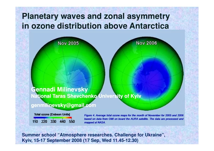
Planetary waves and zonal asymmetry i di t ib ti b A t ti in ozone distribution above Antarctica

Gennadi Milinevsky Gennadi Milinevsky

National National Taras Taras Shevchenko University of Kyiv Shevchenko University of Kyiv genmilinevsky@gmail.com genmilinevsky@gmail.com

Summer school “Atmosphere researches. Challenge for Ukraine”, Kyiv, 15-17 September 2008 (17 Sep, Wed 11.45-12.30)

Ozone hole discovery

May 1985

Antarctic total ozone ground based measurements with Dobson, Brewer , spectrophotometers

Faraday/Vernadsky

Total ozone ground based measurements with Dobson, Brewer spectrophotometers and filter , p p

• zonometers

Fioletov et al., JGR, 2008

Ozonesonde at Halley Station, Antarctica

Shanklin, 2006

Noctilucent (‘night-shining’) Clouds are an indicator of extremely cold conditions in the indicator of extremely cold conditions in the upper atmosphere

Shanklin, 2006

2008: 50 hPa minimum temperature

• 78С
• 85С

NASA

Total ozone measurements by Total ozone measurements by Dobson spectrophotometer at Vernadsky Dobson spectrophotometer at Vernadsky

Ozone measurements 2002-2003 season

Ozone hole development

Total ozone content by Total Ozone M i a b Mapping Spectrometer measurements measurements Nimbus-7, Meteor-3, Earth Probe c d Earth Probe (Aura, OMI since 2004) Ozone 15 September: a) 1980; b) 1990; c) 2000; d) 2005. 2004) p ) ; ) ; ) ; )

Ozone hole area 1980 - 2006

GAW/NASA

WMO, 2006

Biggest in area ozone hole 24 Sept 2006

O h l Ozone hole 14 September 2008

Halley total ozone and 100 hPa temperature 1957 - 2007

100 hPa – 16 km Shanklin, 2007

Faraday/Vernadsky total 1957 - 2005

Shanklin, 2007

Total ozone content trend according Faraday/Vernadsky observations

Season mean data: decreasing since 1980 is b d

• bserved

Main idea: Planetary waves impact on long-term Main idea: Planetary waves impact on long term

total ozone distribution in Antarctica Task:

Analysis of interannual and decadal changes of the quasi- y g q stationary wave amplitude and structure of zonal ozone distribution using the TOMS and partly Dobson Vernadsky t ti d t station data. Time interval: 1979-2005. Season: the spring months September-November. Analysis method: zonal wave parameters determination Analysis method: zonal wave parameters determination using longitudinal distribution of the total ozone at individual latitude circles within 50°S-80°S. latitude circles within 50 S 80 S.

Dataset: TOMS measurements of total ozone content TOMS measurements of total ozone content

http://toms.gsfc.nasa.gov Akademik Vernadsky

Total ozone distribution on 1.10.1979 and 1.10.2004 Regular satellite measurements of total ozone content (TOC) have been carried out using TOMS (Total Ozone Mapping Spectrometer) since 1978 (with a gap in 1993-95) Spatial resolution is equal 1° on since 1978 (with a gap in 1993-95). Spatial resolution is equal 1 on latitude and 1.25° on longitude.

Data base

• 1. Matrix-type database

d d f TOMS produced from TOMS measurements

• 2. Database of secondary

y

• zone distribution

characteristics ( TOC zonal di t ib ti lit d distribution, amplitudes, phase of planetary waves) Longitude –time visualization method visualization method

Fourier analysis

TOC according TOMS data along 65°S 15 October 1996 along 65 S, 15 October 1996 a Zonal number m = 1 – 5 b Zonal number m = 1 5 b Observed and restored total c Obse ed a d esto ed tota

• zone distribution

The first five harmonics give c The first five harmonics give error less then ~3%.

Wavelet analysis

Ti l li ti f Time localization of periodicity TOC periodicity, 2002/03 season June - May Mother wavelet – Morlet function:

( )

2 / 2

( )

2 / 2 cos5

t

t e t ψ

−

= ⋅

Software for visualization of daily and monthly mean ozone TOMS measurements monthly mean ozone TOMS measurements

Ozone hole edge deformation by planetary waves

55 – 70°S latitudes – edge

• f polar vortex, ozone hole

d edge Significant zonal asymmetry due to planetary wave due to planetary wave activity is observed

Planetary waves in total ozone

Total ozone distribution to the south Total ozone distribution to the south

• f 30°S, 25.09.2001. Dashed line

marks the latitude circle 65°S. Traveling wave from ground-based Traveling wave from ground based

• bservations.

Planetary waves in total ozone distribution (ozone hole edge deformation) ( g )

Planetary waves with zonal wave numbers m = 1, 2, 3

Planetary waves in total ozone

ember m 1 Septe Days fro

1979 1988 2003

Longitude Longitude Longitude

1979 1988 2003

Longitude – time visualization of ozone distribution

• g tude

t e sua at o

• o o e d st but o

(65°S) (Hovmöller diagram)

Quasi stationary and traveling waves y g

Traveling wave wave TOC for 65 S, September - November 1996 , p

Quasi stationary wave Quasi stationary wave

Increasing of ozone t i i

Monthly mean longitudinal

asymmetry in spring

Monthly mean longitudinal distributions of the total ozone by the TOMS data for (a) the 9 months of the southern summer, autumn and winter 2005 at 60°S; 60 S; (b) the spring months September, October and November 2005 at 60°S.

Climatology of the total ozone asymmetry

• ver Antarctica 1979-2005
• ver Antarctica, 1979 2005
• the polar low ozone anomaly;

eastward shift by about 45° in ozone minimum position (blue) and

• eastward shift by about 45 in ozone minimum position (blue) and

relatively stable position of zonal maximum (red)

Geographical position of zonal extremes in total ozone in total ozone

The average positions of the quasi-stationary extremes in September- November 1979-2005 (left) and the 5-year means for 1979-1983 and 2001- November 1979 2005 (left) and the 5 year means for 1979 1983 and 2001 2005 (right). At high latitudes the positions of maximum outline the continent boundary in region of Victoria Land and Wilkes Land. Minima are located along Antarctic Peninsula in average data of 1973 1983 and shift eastward along Antarctic Peninsula in average data of 1973-1983 and shift eastward during last decades. Shift distance is about 45°, or ∼ 2000 km at 65 °S.

Ozone distribution asymmetry in the Southern Hemisphere Southern Hemisphere

Ozone hole (blue) and ozone Ozone hole (blue) and ozone rich collar (red) take typically asymmetric positions relative to the South pole due to to the South pole due to quasi-stationary planetary waves influence.

Fig 1 October mean fields of the

• Fig. 1. October mean fields of the

total ozone, 45°S -90°S,TOMS

• data. The dashed circle marks the

latitude 65°S By Grytsai et al. (2007), Ann. latitude 65 S. y y ( ), Geophys., 25 (2), 361–374, Fig. 1.

Empirical Orthogonal Function (EOF) analysis of NCEP tropopause temperature y p p p

1979-2007 September 9 9 00 Septe be the spatial variability of the leading EOF in monthly mean tropopause temperature

Definitions

Tropopause is a boundary between turbulent troposphere, in which the temperature decreases with height, and stratified stratosphere where temperature increases with height. Tropopause elevation takes place when stratosphere cools p p p p (left) or troposphere warms (right).

Stratosphere impact Troposphere impact by (Shepherd, JMS of Japan, 2002)

Total ozone and tropopause zonal anomalies

Total ozone content d t and tropopause height anti- correlates. Spring Antarctic tropopause is p p influenced by the lower stratosphere temperature formed temperature formed by ozone distribution.

Monthly mean eddy fields of (a b) total ozone and (c d) tropopause Monthly mean eddy fields of (a, b) total ozone and (c, d) tropopause height by TOMS/OMI data and NCEP-NCAR reanalysis data, respectively.

Stratospheric impact on tropopause position

Longitudinal distribution Longitudinal distribution

• f (a) total ozone, (b)

tropopause pressure/height along the latitude circle 65°S f O t b 2006 for October 2006. Strong anti-correlation between tropopause height and total ozone content shows that ozone losses are a cause total ozone content shows that ozone losses are a cause

• f the spring tropopause elevation in Antarctic region.

Tropopause trend asymmetry p p y y

In average, the highest tropopause pressure trends are are 1979-2006: -7±3 hPa/dec. 1979-2000: -17±4 hPa/dec.

• r ∼0.5 km/dec.

(at the level of ±1σ). About zero trends are observed in

• zone collar region
• zone collar region.

Difference in tropopause pressure/height trends over the Difference in tropopause pressure/height trends over the regions of total ozone extremes.

Tropopause sharpness decrease i i i TOC i i in spring in TOC min region

Eddy tropopause pressure monthly pressure monthly mean, Oct 2005

Vertical temperature profiles in spring 2005 for the tropopause zonal extremes at latitude 65°S, longitudes 30°W (tropopause zonal extremes at latitude 65 S, longitudes 30 W (tropopause height maximum) and 150°E (tropopause height minimum).

Meridional tropopause structure

Four meridional planes along which tropopause profiles “equator pole equator” for equator-pole-equator for Southern Hemisphere have been

• btained.
• btained.

A l Anomalous tropopause height Tropopa se press re/height profiles for The tropopause elevation Tropopause pressure/height profiles for October 2005 in the four meridional directions. is observed in Atlantic sector.

Tropopause seasonal variations

Anomalous tropopause height Tropopause pressure/height profiles for 4 p seasons of 2005 meridional section section 45°W-135°E

Anomalous tropopause elevation occurs during winter and

• spring. Other seasons are characterized by uniform

h i h di ib i A i R i tropopause height distribution over Antarctic Region. Disturbed tropopause height equals 13-14 km (JJA, SON). Typical undisturbed values reach only 9 km (DJF, MAM).

1968-1996 July-December Long-term means eddy fields by NCEP-NCAR reanalysis hPa

• 2.4
• 2.1
• 5.2
• 6.8
• 6.1
• 1.5

JULY DECEMBER AUGUST SEPTEMBER OCTOBER NOVEMBER

100 3.2 3.2 5.6 8.2 6.5 1.8 100 hPa, mean eddy temperature, K popause

• 29
• 26

28 28 25 33 32 23

• 27
• 29
• 26
• 19

Mean tropopause pressure, hPa eddy Tro a

• 2.4

25 33 32 7 hPa 00 12

• 15

5.1 -6.2 3.2 2.4

• 23

16

• 22

16

• 22

17

Winter-spring zonal anomalies in troposphere temperature

700 hPa, mean eddy temperature, K

p g p p p (bottom), tropopause pressure (middle) and lower stratosphere temperature (top) by the long-term means of 1968-1996.

Scheme of Antarctic troposphere and stratosphere contribution to formation of tropopause meridional profile

Stratosphere influence in winter p T h i fl i d i i Troposphere influence in summer and in winter Asymmetric Antarctic continent

Large-scale Brewer-Dobson circulation g

cross-tropopause exchange cross tropopause exchange quasi-horizontal transport

Normal Brewer-Dobson circulation (North ( Hemisphere, by Holton et al., 1995)

Exchange trough Exchange trough antarctic tropopause due to regional slope of meridional profile in winter and spring

Possibility of horizontal cross-tropopause exchange in the region of elevated exchange in the region of elevated tropopause over West Antarctica

I bi ti ith f diti

Conclusions: tropopause

In combination with surface conditions, the changes of tropopause structure could impact to regional troposphere could impact to regional troposphere state:

• increase of troposphere thickness

decrease of tropopause sharpness

10 e, hPa 30 20 km Transition layer

• decrease of tropopause sharpness

and modification of vertical troposphere/stratosphere exchange

80 60 40 20 100 1000 Pressure 10 Height, Transition layer

troposphere/stratosphere exchange

• increase of possibility the cross-
• 80 -60 -40 -20 0

tropopause horizontal transport modification of planetary wave

• modification of planetary wave

propagation

Task home message Task-home message -

• zone

Changes in ozone max and min positions:

• how impact on ecosystem due to redistribution of

UV radiation at sea level UV radiation at sea level

• how influence on regional climate
• what is the future of ozone hole