Performance What do we mean by Performance? We must take many - - PowerPoint PPT Presentation

94 CSE378 WINTER, 2001

Performance

95 CSE378 WINTER, 2001

What do we mean by Performance?

• We must take many different factors into account:
• Technology
• basic circuit speed (clock speed, usually in MHz: millions of

cycles per second, now in GHz: billions of cycles per sec.)

• process technology (how many transistors on a chip)
• Organization
• what style of ISA (RISC or CISC)
• what type of memory hierarchy
• how many processors in the system
• Software
• quality of the compiler, OS, database driver, etc...
• There’s alot more to measuring performance than clock speed...

96 CSE378 WINTER, 2001

Metrics

• Raw speed (peak performance, but it is never attained)
• Execution time (also called response time, i.e. time to execute one

program from beginning to end). Need specific benchmarks for:

• Integer dominated programs (compilers, etc)
• Scientific (lots of floating point usage)
• Graphics/multimedia
• Throughput (total amount of work in given time)
• Good metrics for systems managers
• Database programs (keeping the most people happy at the

same time)

• Often, improving execution time will improve throughput, and vice

versa.

97 CSE378 WINTER, 2001

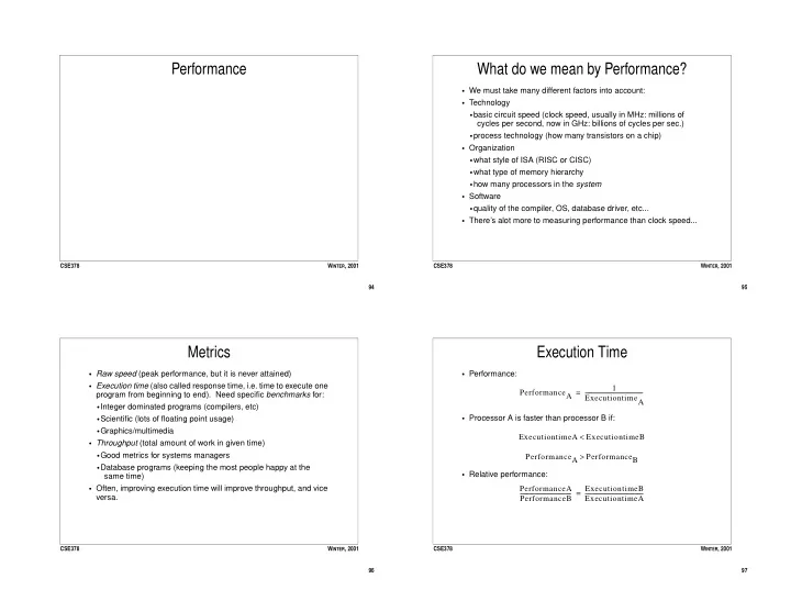
Execution Time

• Performance:
• Processor A is faster than processor B if:
• Relative performance:

PerformanceA 1 ExecutiontimeA

• =

ExecutiontimeA ExecutiontimeB < PerformanceA PerformanceB > PerformanceA PerformanceB

• ExecutiontimeB

ExecutiontimeA

• =

98 CSE378 WINTER, 2001

Measuring Execution Time

• Wall clock, response time, elapsed time
• Unix time function:

[tahiti]:~ % time someprogram 346.085u 0.394s 5:48.32 99.4% 5+302k 0+0io 0pf+0w

• “time” lists User CPU time, System CPU time, elapsed time,

percentage of elapsed time which is total CPU time, as well as information about the process size, quantity of IO, etc.

• Because of OS differences, it is hard to make comparisons from
• ne system to another...
• For the remainder of this lecture, we’ll use User CPU time to

mean CPU execution time (or just execution time)

99 CSE378 WINTER, 2001

Definition of CPU Execution Time

• CPU Execution Time = CPU clock cycles x clock cycle time
• CPU execution time is program dependent
• CPU clock cycles is program dependent
• clock cycle time (usually in nanoseconds, ns) depends on the

particular machine

• Since clock cycle time = 1/clock cycle rate (clock cycle rate is in

MHz, millions of cycles per second) an alternate definition is: CPU Execution Time CPU clock cycles clock cycle rate

• =

100 CSE378 WINTER, 2001

CPI - Cycles Per Instruction

• Definition: CPI is the average number of clock cycles per

instruction.

• CPI in isolation is not a measure of performance (program and

compiler dependent)

• Ideally, CPI = 1, but this might slow down the clock (compromise)
• CPI can (and usually is) greater than 1 because of breaks in

control flow and the impact of the memory hierarchy

• Can we have CPI < 1?

CPU clock cycles Number of Instructions CPI × = CPU Exec Time Number of Instructions CPI × clock cycle time × =

101 CSE378 WINTER, 2001

Class of Instructions

• You can give different CPIs for various classes of instructions (e.g.

floating point arithmetic instructions take longer than integer instructions, load-store instructions take longer than logical instructions, etc.)

• Ci is the number of instructions in the ith class that have been

executed

• Note that minimizing the number of instructions does not

necessarily improve the execution time of the program

• Improving part of the architecture can improve a Cj. We often talk

about the contribution to CPI of a certain class of instructions. CPU Exec time CPIi Ci × ( )

1 n

∑

clock cycle time × =

102 CSE378 WINTER, 2001

Measuring average CPI

• Instruction count: need a simulator or (possibly less precise) a

profiler

• Simulator “interprets” every instruction and counts them
• Profiler can either count how many times each basic block has

been executed or use some sampling technique

• CPU Execution time can be measured (elapsed time)
• Clock cycle time is given by the processor
• We know execution time, cycle time, so we can solve for total

cycles.

• Knowing the total cycles together with the total number of

instructions executed lets us solve for average CPI.

103 CSE378 WINTER, 2001

Other Popular Metrics - MIPS

• MIPS = Millions of Instructions Per Second
• r
• Since MIPS is a rate, the higher the better.
• But MIPS in isolation is no better than CPI in isolation. MIPS is:
• Program dependent
• Does not take the instruction set into account (CISC programs

will typically take fewer instructions than RISC, so we can’t compare different ISAs) MIPS Instruction Count Exec time

6

×10

• =

MIPS clock rate CPI

6

×10

• =

104 CSE378 WINTER, 2001

The Trouble with MIPS

• Using MIPS can give “wrong” results:
• Machine A with compiler C1 executes program P in 10 seconds,

using 100,000,000 instructions (10 MIPS)

• Machine A with compiler C2 executes program P in 15 seconds,

using 180,000,000 instructions (12 MIPS)

• While C1 is clearly faster than C2, C1 has a lower MIPS rating

than C2....

• ... the trouble with MIPS is that it doesn’t take CPI into account.

105 CSE378 WINTER, 2001

Other Popular Metrics - MFLOPS

• MFLOPS = Millions of floating point operations per second
• Same problems as MIPS:
• Program dependent
• Doesn’t take instruction set into account
• Counts operations, not the time to execute them...

MFLOPS Number of floating point instructions Exec time

6

×10

• =

106 CSE378 WINTER, 2001

Benchmarks

• Benchmarks: workload representative of what the computer will

actually be used for.

• Industry benchmarks to compare machines: SPEC benchmarks

(SPECint, SPECfp), Perfect Club

• Database benchmarks
• Multimedia benchmarks
• Caveats:
• Compilers optimize specifically for benchmarks
• Old SPEC benchmarks (1992) were too small (didn’t test the

memory system sufficiently)

• Utilities, user interface, etc. are often not in benchmarks

107 CSE378 WINTER, 2001

Amdahl’s Law

• The amount that we can improve performance with a given

improvement is limited by the amount that the improved feature is actually used:

• For instance, if loads/stores take up 33% of our execution time,

how much do we need to improve loads/stores to make the program run 1.5 times faster?

• Important corollary: Make the common case fast.

Exec time after improvement Exec time affected by improvement Amount of improvement

• Exec time unaffected

+ = 108 CSE378 WINTER, 2001

Example Measurements

• What is the average CPI for gcc? For spice? Should we expect

CPI for a given category to be the same btwn two programs?

Instruction Category GCC SPICE

• Ave. CPI

Load/Store 33% 40% 1.4 Branch 16% 8% 1.8 Jumps 2% 2% 1.2 FP Add

• 5%

2.0 FP Sub

• 3%

4.0 FP Mul

• 6%

5.0 FP Div

• 3%

19.0 Other (Integer add/sub, stl, etc) 49% 33% 1.0

109 CSE378 WINTER, 2001

Evolution of ISAs

110 CSE378 WINTER, 2001

Characterizing ISAs

• A traditional way to look at ISA complexity encompasses:
• Number of operands per instruction:
• How many operands are specified in an instruction?
• Is the number of operands fixed?
• Number of addresses per instruction: How many of the operands

can be memory addresses?

• Regularity of instruction formats:
• Variable length or fixed length?
• Few or many formats?
• Number of addressing modes/types.
• Registers
• Special purpose (reserved) or general purpose?
• Are the registers implied/specified in the instruction?

111 CSE378 WINTER, 2001

A Tour of Common Addressing Modes

• We use VAX-like asm notation for non-MIPS addr modes...

Name Example Meaning * Immediate 100 100 * Register r6 Contents of r6 Register Deferred (r6) Memory[r6] * Based/Displacement 100(r6) Memory[r6+100] * PC-Relative 100 PC + 100 Deferred @100(r6) Memory[Memory[r6+100]] Autoincrement (r3)+ Memory[r3]; r3 = r3 + size Autodecrement

• (r3)

r3 = r3 - size; Memory[r3] Autoincrement deferred @(r3)+ Memory[Memory[r3]]; r3 = r3 + size

112 CSE378 WINTER, 2001

Accumulator Machines

• Early machines, and many microcontroller (Motorola 6802) used

an implied register called an accumulator.

• Operands per instruction: at most 1
• Addresses per instruction: at most 1
• Instruction formats: fixed length, few formats for ease of

programming

• Addressing modes: few (typically immediate and and PC-

relative)

• Registers: one implied register
• How would we encode A = B + C; ?

load addressB add addressC store addressA

113 CSE378 WINTER, 2001

Stack Machines

• Machines where all data is on an implied stack
• Operands per instruction: at most 1
• Addresses per instruction: at most 1
• Instruction formats: variable length, few formats
• Addressing modes: few (typically immediate and and PC-

relative)

• Registers: none (for performance, there are often “hidden”

registers)

• How would we encode A = B + C; ?

push addressB push addressC add pop addressC

114 CSE378 WINTER, 2001

CISC Machines

• Intel 80x86, Motorola 680x0 are examples of CISC machines.
• They are register-memory architectures (a few operands are

allowed to be memory addresses)

• Operands per instruction: variable, up to 2
• Addresses per instruction: 1
• Instruction formats: variable length (80x86 instructions are

between 1 and 6 bytes), many formats

• Addressing modes: 80x86 has at least 7, 68k has more
• Registers: usually a few special purpose and a few general

purpose (80x86 has 8 special purpose, 8 fp; 680x0 has 8 data, 8 address)

• How would we encode A = B + C; ?

load r1, addressB add r1, addressC store r1, addressA

115 CSE378 WINTER, 2001

True CISC

• The VAX is the ultimate CISC.
• Operands per instruction: variable, up to 3
• Addresses per instruction: variable, up to 3
• Instruction formats: variable length (1 to 54 bytes), many formats
• Addressing modes: more than 10
• Registers: 16 general purpose
• How would we encode A = B + C; ?

add addressA, addressB, addressC

• VAX also included special loop instructions, as well as call and

return instructions

• Compared to the one MIPS add instruction, VAX has many

versions, depending on # of operands and addressing modes, leading to thousands of different combinations.

• This complicates the implementation of the processor

tremendously.

116 CSE378 WINTER, 2001

RISCs

• Typically load-store or register-register architectures
• Operands per instruction: 3
• Addresses per instruction: 0 (must use load/store operations to

move data between memory and registers)

• Instruction formats: fixed length, few formats
• Addressing modes: few (MIPS has immediate, register, based,

and PC-relative)

• Registers: many general purpose
• How would we encode A = B + C; ?

lw r1, offsetA(r5) lw r2, offsetB(r5) add r3, r2, r1 sw r3, offsetC(r5)

117 CSE378 WINTER, 2001

Summary Comparisons

• If RISCs have high instruction count, how can they possibly

achieve such good performance?

Accumulator Stack CISC RISC Implementation easy easy hard easy Instruction density high high high low Assembly coding easy medium easiest tiresome Compilation easy easy easy hard Memory overhead high high highest? lower Instruction count medium medium low high CPI medium medium high low Cycle time ? ? high low

118 CSE378 WINTER, 2001

Historical Trends

• The 60s: expensive memory, poor compiler technologies, poor

implementation technologies.

• Goals: simple compilers (or assembling), simple hardware

implementation, high code density

• Results: simple ISA, regular formats, compact encoding
• The 70s: advances in implementation technologies, poor

compilers, expensive memory, high software costs

• Goals: simple compilers, high code density
• Results: powerful ISA, irregular formats, compact encoding,

complicated implementations

• The 80s saw advances in implementation tech, advanced

compilers, cheap memory

• Goals: high performance by pipelining, simple implementation,
• compat. w/ optimizing compilers
• Results: simple ISA, regular formats, lots of registers

119 CSE378 WINTER, 2001

Some Modern Processors

Processor Mhz Year Style Trans. x 106 SpecInt/Fp92 SpecInt/Fp95 Intel 386DX 33 1987 CISC 0.275 8/3 R3000 40 1988 RISC 0.3 28/36 Motorola 68040 25 1989 CISC 1.2 21/15 Intel 80486DX 50 1991 CISC 1.2 33/15 R4400 250 1995 RISC 2.2 180/180 Intel P6 166 1996 CISC 5.5 ~290/260 ~7/6 Dec Alpha 21164 300 1995 RISC 9.3 ~330/500 ~9/13 Intel PIII 1000 2000 CISC 28 ~1800/1800 ~45/45 SPARC Ultra III 900 2000 RISC 28 ~2000/3000 ~50/90