Partial Matching between Surfaces U i Using Frchet Distance F h t - - PowerPoint PPT Presentation

partial matching between surfaces u i using fr chet
SMART_READER_LITE
LIVE PREVIEW

Partial Matching between Surfaces U i Using Frchet Distance F h t - - PowerPoint PPT Presentation

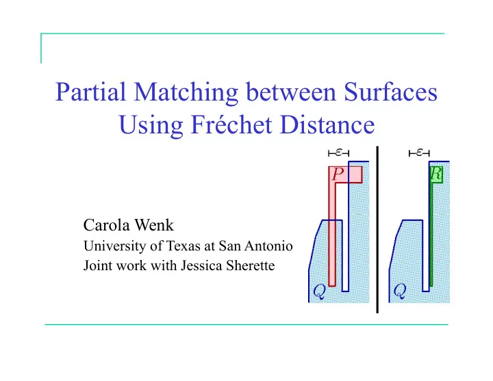
Partial Matching between Surfaces U i Using Frchet Distance F h t Di t Carola Wenk University of Texas at San Antonio J i t Joint work with Jessica Sherette k ith J i Sh tt Geometric Shape Matching p g Consider geometric


slide-1
SLIDE 1

Partial Matching between Surfaces U i F é h t Di t Using Fréchet Distance

Carola Wenk

University of Texas at San Antonio J i t k ith J i Sh tt Joint work with Jessica Sherette

slide-2
SLIDE 2

Geometric Shape Matching p g

  • Consider geometric shapes

to be composed of a number f b i bj

  • f basic objects

such as points line segments triangles

  • How similar are two

geometric shapes?

  • Choice of distance measure
  • Full or partial matching
  • Full or partial matching
  • Exact or approximate matching
  • Transformations (translations, rotations, scalings)

( , , g )

slide-3
SLIDE 3

Shape Matching - Applications

  • Character Recognition
  • Fingerprint Identification
  • Molecule Docking, Drug Design

g, g g

  • Image Interpretation and Segmentation
  • Quality Control of Workpieces

Quality Control of Workpieces

  • Robotics
  • Pose Determination of Satellites
  • Pose Determination of Satellites
  • Puzzling
  • . . .
slide-4
SLIDE 4

Distance Measures

  • Directed Hausdorff distance

δ

→(A B)

i || b || A B δ (A,B) = max min || a-b ||

  • Undirected Hausdorff-distance

→ →

A B δ

→(B,A)

δ

→(A B)

a ∈A b∈B

δ(A,B) = max (δ

→(A,B) , δ →(B,A) )

But: δ (A,B) But:

  • Small Hausdorff distance
  • When considered as curves the

distance should be large

  • The Fréchet distance is well-suited to

i h compare continuous shapes.

slide-5
SLIDE 5

Fréchet Distance for Curves

δF(f,g) = inf max ||f(t)-g(σ(t))||

σ:[0,1] [0,1] t ∈[0,1]

f,g: [0,1] → R2

[ , ] [ , ] [ , ]

where α and β range over continuous monotone increasing reparameterizations only.

  • Man and dog walk on

p y g

  • ne curve each
  • They hold each other at

a leash

  • They are only allowed

f

to go forward

  • δF is the minimal

ibl l h l th

g

possible leash length

[F06] M. Fréchet, Sur quelques points de calcul fonctionel, Rendiconti del Circolo Mathematico di Palermo 22: 1-74, 1906.

slide-6
SLIDE 6

Free Space Diagram

g g >ε f f ≤ε

  • Fε(f,g) = { (s,t)∈[0,1]2 | || f(s) - g(t)|| ≤ ε } white points

free space of f and g f p g

slide-7
SLIDE 7

Free Space Diagram

g α g β f f

  • Fε(f,g) = { (s,t)∈[0,1]2 | || f(s) - g(t)|| ≤ ε } white points

free space of f and g p g

  • δF(f,g) ≤ ε iff there is a monotone path in the free space from

(0,0) to (1,1)

  • Can be decided using DP in O(mn) time [AG95]

[AG95] H. Alt, M. Godau, Computing the Fréchet distance between two polygonal curves, IJCGA 5: 75-91, 1995.

slide-8
SLIDE 8

Fréchet Distance for Surfaces

  • Given: Two surfaces

P,Q: [0,1]2→ Rd

  • The Fréchet distance is defined as:

P Q δF(P,Q) = inf max ||t-σ(t)||

σ:P→Q σ homeomorphism t∈P

  • Is δF (P,Q) = δF (∂P, ∂Q)?

No: δF (∂P, ∂Q) ≈ w/2 δ (P Q) h/2 h δF (P,Q) ≈ h/2 w

[BBW08] K. Buchin, M. Buchin, C. Wenk, Computing the Fréchet Distance Between Simple Polygons, CGTA 41: 2-20, 2008.

slide-9
SLIDE 9

Fréchet Distance for Surfaces

  • For piecewise linear surfaces:
  • Computing δF is NP-hard, even when one surface is a triangle,
  • r when both surfaces are polygons with holes or terrains
  • δF is upper-semi-computable; it is unknown if it is computable

[G98] [BBS10] [AB09]

δF is upper semi computable; it is unknown if it is computable

  • For simple polygons:
  • δF can be computed in polynomial time

[BBW08]

  • Partial δF can be decided in polynomial time
  • For folded polygons:

[SW12] [C S 11] • δF can be approximated in polynomial time

[BBS10] K. Buchin, M. Buchin, A. Schulz, Fréchet distance for surfaces: Some simple hard cases, ESA: 63-74, 2010. [SW12] J. Sherette, C. Wenk, Computing the Partial Fréchet Distance Between Polygons, SWAT, 2012. [CDHSW11] A F Cook IV A Driemel S Har Peled J Sherette C Wenk Computing the Fréchet Folded Polygons WADS 2011

[CDHSW11]

[BBW08] K. Buchin, M. Buchin, C. Wenk, Computing the Fréchet Distance Between Simple Polygons, CGTA 41: 2-20, 2008. [G98] M. Godau, On the complexity of measuring the similarity…, Dissertation, Freie Universität Berlin, 1998. [AB09] H. Alt, M. Buchin, Can we compute the similarity between surfaces?, D&CG, to appear. [CDHSW11] A.F.Cook IV, A. Driemel, S. Har-Peled, J. Sherette, C. Wenk, Computing the Fréchet….Folded Polygons,WADS, 2011.

slide-10
SLIDE 10

Partial Fréchet Distance

  • Given: Two simple polygons P, Q (coplanar, triangulated),

and some ε>0.

  • Task: Decide whether there exists a simple polygon R ⊆ Q

such that δF(P,R) ≤ ε .

  • P⊆Q

⇒ R=P, ε=0

  • P∩Q = ∅

⇒ Similar to proj- ecting P to ∂Q

  • Points in P∩Q are not

mapped straight down M i f i i ecting P to ∂Q

  • Mapping of points is

not independent from

  • ther points
slide-11
SLIDE 11

Approach for Fréchet Distance b t Si l P l between Simple Polygons

P Q

a’ c’

Restrict the homeomorphisms: Map diagonals in P only to For ε>0, find homeom. such that:

a b’ c

σ

b

Map diagonals in P only to shortest paths in Q. For ε 0, find homeom. such that:

  • 1. δF(∂P,∂Q) ≤ ε

(specifies mapping for

  • 2. Every diagonal D in P has

distance ≤ ε to corresponding diagonal endpoints) shortest path in Q Map boundary & check diagonals: Comp te combinatoriall eq i alent mappings from ∂P to ∂Q This yields a polynomial time algorithm Compute combinatorially equivalent mappings from ∂P to ∂Q, that also ensure small δF between diagonals and shortest paths

[BBW08] K. Buchin, M. Buchin, C. Wenk, Computing the Fréchet Distance Between Simple Polygons, CGTA 41: 2-20, 2008.

This yields a polynomial-time algorithm.

slide-12
SLIDE 12

(Double) Free Space Diagram

  • Free space diagram: ∂P×∂Q

Free space diagram: ∂P ∂Q

  • Boundary mapping from ∂P to ∂Q corresponds to a monotone

path from bottom to top (that maps all of P).

slide-13
SLIDE 13

Approach for Partial Fréchet Distance b t Si l P l between Simple Polygons

  • Since we have to find R⊆Q, the boundary of R is not known.

⇒ Cannot just map boundaries anymore ⇒ Cannot just map boundaries anymore.

  • We extend simple polygons approach in a different way:

1 Map boundary & check diagonals:

  • 1. Map boundary & check diagonals:

Compute combinatorially equivalent mappings from ∂P to ∂Q some closed curve in Q, that also ensure small δF between Q

F

diagonals and shortest paths . ⇒ (Q,ε)-valid set of neighborhoods

2 Construct R from (Q ε) valid set

  • 2. Construct R from (Q,ε)-valid set

Prove that a (Q,ε)-valid set of neighborhoods always contains a valid simple polygon R⊆Q p p yg ⊆Q

slide-14
SLIDE 14

3D Free Space Diagram

  • Free space diagram: ∂P×Q
  • Sequence of slices p ×Q
  • Sequence of slices pi×Q
  • Boundary mapping from ∂P to closed curve in Q corresponds to a

monotone path from first slice to last slice.

  • Note: Path need only be monotone along P.
slide-15
SLIDE 15

Reachability

Pair of adjacent slices in free space diagram: Scenario in Q: i h bl f iff δ ( ( ))

  • a2 is reachable from a1 iff δF(p3p4, π(a1,a2)) ≤ ε,

where π(a1,a2) is the shortest path in Q between a1 and a2.

  • a2 is reachable from a1, but a3 is not.

2 1, 3

slide-16
SLIDE 16

Neighborhoods

  • ε-disk Dε(p3).
  • Points in Dε(p3)∩Q can be

d t

  • Neighborhood of pi:

Maximal connected subset of D (p )∩Q mapped to p3. Dε(pi)∩Q

slide-17
SLIDE 17

Propagate Reachability

Pair of adjacent slices in free space diagram: Scenario in Q: N4 N3 i h bl f iff δ ( ( )) N3

  • a2 is reachable from a1 iff δF(p3p4, π(a1,a2)) ≤ ε,

where π(a1,a2) is the shortest path in Q between a1 and a2.

  • All points in one neighborhood are reachable from all points in

p g p another neighborhood, if there exists one reachable pair of points.

  • Compute reachability between two neighborhoods in O(n) time.
slide-18
SLIDE 18

Algorithm: Neighborhoods

  • Each slice contains at most

O(n) neighborhoods per point point.

  • There are O(n2) pairs of

neighborhoods to test g reachability between, for each pair of slices.

slide-19
SLIDE 19

Algorithm: Neighborhoods

  • There are O(m) slices,

where m=|P|

  • We can compute and
  • We can compute and

propagate reachability through free space diagram g p g in O(n3 m) time

  • ⇒ Test whether a reachable

th i t d t t path exists, and construct valid set of neighborhoods, in polynomial time. p y

slide-20
SLIDE 20

Slight Modification

  • So far we have only mapped ∂P,

but we have not considered the

  • Modify algorithm, by merging

slices in a different order: diagonals of P yet.

  • Locally from left to right
  • Merge in diagonal-nesting-
  • rder
  • rder
slide-21
SLIDE 21

Approach for Partial Fréchet Distance b t Si l P l between Simple Polygons

  • Since we have to find R⊆Q, the boundary of R is not known.

⇒ Simply mapping boundaries does not work ⇒ Simply mapping boundaries does not work.

  • We extend simple polygons approach in a different way:

1 Map boundary & check diagonals:

  • 1. Map boundary & check diagonals:

Compute combinatorially equivalent mappings from ∂P to ∂Q some closed curve in Q, that also ensure small δF between Q

F

diagonals and shortest paths . ⇒ (Q,ε)-valid set of neighborhoods

2 Construct R from (Q ε) valid set

  • 2. Construct R from (Q,ε)-valid set

Prove that a (Q,ε)-valid set of neighborhoods always contains a valid simple polygon R⊆Q p p yg ⊆Q

slide-22
SLIDE 22

Finding R

  • A valid set of neighborhoods
  • We want to compute a simple

We w

  • co pu e

s p e polygon R that maps every pi to a point in its associated neighborhood. neighborhood.

slide-23
SLIDE 23

Finding R

  • We iteratively construct R by

mapping each pi to a point in its associated neighborhood.

  • At each iteration:
  • We show that the points can
  • We show that the points can

be mapped to form a simple polygon. W ll i i t

  • We allow remapping points

within their neighborhood.

  • By properties of the

neighborhoods, δF stays ≤ ε

slide-24
SLIDE 24

Finding R

  • Initially, choose one triangle in P.
  • Map each point a in its associated

p e c po s ssoc ed neighborhood Na.

  • In each iterative step, add points

which are connected to already which are connected to already mapped points.

  • If the neighborhood does not

t i th i i l i t it contain the original point, map it inside Q and connect previous points with shortest paths.

slide-25
SLIDE 25

Finding R

  • If adding a point and a shortest

path yields a self-intersection:

  • The neighborhood around a

previous point is crossed.

  • We need to remap to a point
  • We need to remap to a point

below the shortest path. ⇒In the end we have found a simple l R polygon R. ⇒ Vertices of P are mapped to points in associated neighborhoods. ⇒Hence, δF(P,R) ≤ ε .

slide-26
SLIDE 26

Original Regions

  • The neighborhoods of points can be split

into multiple disjoint parts by R.

  • We must choose one of these two regions

to map a to.

  • Unfortunately an arbitrary choice may be invalidated by a later

mapping of R mapping of R.

slide-27
SLIDE 27

Original Region

  • The key idea is to map a point a’
  • n the same side (relative to R)

as a is to the preimage of that portion of R. ⇒ Original region

slide-28
SLIDE 28

Conclusions:

  • We presented the first algorithm for computing

partial FD between surfaces. This algorithm runs p g in polynomial time.

  • In the future it would be interesting to consider

th i t f ti l FD

  • ther variants of partial FD.
  • It would also be interesting to consider

extending this algorithm other classes of surfaces extending this algorithm other classes of surfaces