Part I 1. Input: detailed information about legs of flight. 2. F : - PowerPoint PPT Presentation

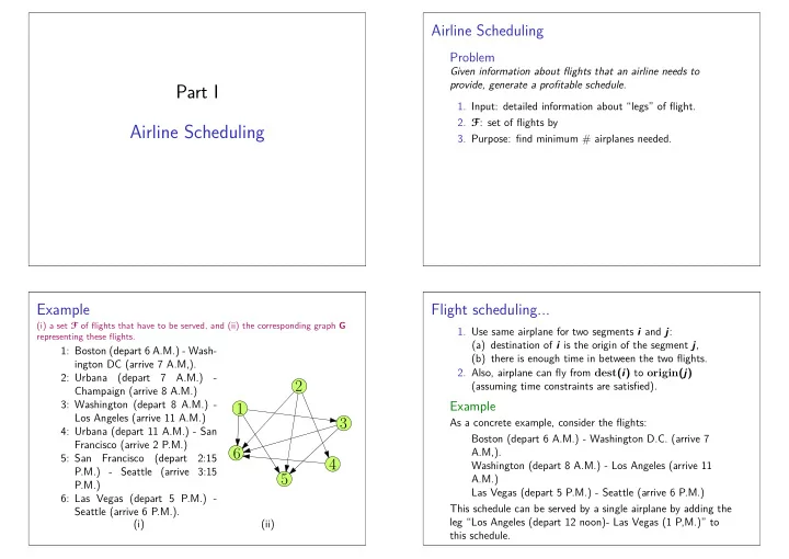
Airline Scheduling Problem Given information about flights that an airline needs to provide, generate a profitable schedule. Part I 1. Input: detailed information about “legs” of flight. 2. F : set of flights by Airline Scheduling 3. Purpose: find minimum # airplanes needed. Example Flight scheduling... (i) a set F of flights that have to be served, and (ii) the corresponding graph G 1. Use same airplane for two segments i and j : representing these flights. (a) destination of i is the origin of the segment j , 1: Boston (depart 6 A.M.) - Wash- (b) there is enough time in between the two flights. ington DC (arrive 7 A.M,). 2. Also, airplane can fly from dest ( i ) to origin ( j ) 2: Urbana (depart 7 A.M.) - 2 (assuming time constraints are satisfied). Champaign (arrive 8 A.M.) 3: Washington (depart 8 A.M.) - Example 1 Los Angeles (arrive 11 A.M.) 3 As a concrete example, consider the flights: 4: Urbana (depart 11 A.M.) - San Boston (depart 6 A.M.) - Washington D.C. (arrive 7 Francisco (arrive 2 P.M.) 6 A.M,). 5: San Francisco (depart 2:15 4 Washington (depart 8 A.M.) - Los Angeles (arrive 11 P.M.) - Seattle (arrive 3:15 5 A.M.) P.M.) Las Vegas (depart 5 P.M.) - Seattle (arrive 6 P.M.) 6: Las Vegas (depart 5 P.M.) - This schedule can be served by a single airplane by adding the Seattle (arrive 6 P.M.). leg “Los Angeles (depart 12 noon)- Las Vegas (1 P,M.)” to (i) (ii) this schedule.

Modeling the problem Solution 1. model the feasibility constraints by a graph. 1. Reduction to computation of circulation. 2. Build graph H . 2. G : directed graph over flight legs. 3. ∀ leg i , two new vertices u i , v i ∈ VH . 3. For i and j (legs), ( i → j ) ∈ E ( G ) ⇐ ⇒ same airplane s : source vertex. t : sink vertex. can serve both i and j . 4. Set demand at t to k , Demand at s to be − k . 4. G is acyclic. 5. Each flight must be served. New edge e i = ( u i → v i ) , 5. Q: Can required legs can be served using only k airplanes? for leg i . Also ℓ ( e i ) = 1 and c ( e i ) = 1 . 6. If same plane can so i and j (i.e., ( i → j ) ∈ E ( G ) ) then add edge ( v i → u j ) with capacity 1 to H . 7. Since any airplane can start the day with flight i : add an edge ( s → u i ) with capacity 1 to H , ∀ i . 8. Add edge ( v j → t ) with capacity 1 to G , ∀ j . 9. Overflow airplanes: “overflow” edge ( s → t ) with capacity k . Let H denote the resulting graph. Example of resulting graph Lemma The resulting graph H for the instance of airline scheduling show before. Lemma ∃ way perform all flights of F ≤ k planes ⇐ ⇒ ∃ circulation k in H . 1 , 1 u 1 v 1 Proof. 1 , 1 u 2 v 2 1. Given feasible solution → translate into valid circulation. 1 , 1 2. Given feasible circulation... u 3 v 3 − k k 3. ... extract paths from flow. 1 , 1 s t u 4 v 4 4. ... every path is a plane. 2 1 , 1 u 5 v 5 1 3 1 , 1 u 6 v 6 6 4 5

Extensions and limitations 1. a lot of other considerations: (i) airplanes have to undergo long term maintenance treatments every once in awhile, Part II (ii) one needs to allocate crew to these flights, (iii) schedule differ between days, and (iv) ultimately we interested in maximizing revenue. Image Segmentation 2. Network flow is used in practice, real world problems are complicated, and network flow can capture only a few aspects. 3. ... a good starting point. Image Segmentation What is the input... 1. Input is a bitmap on a grid. Input is an image. 2. Every grid node represents a Partition image into background and foreground. pixel 3. Convert grid into a directed graph G , 4. Input: (i) N × N bitmap. G = ( V , E ) . (ii) ∀ pixel i : foreground value (i) (ii) f i ≥ 0 . The (i) input image, and (ii) a possible segmentation of the (iii) ∀ pixel i : background image. value b i . (iv) ∀ i , j adjacent: separation penalty p ij . (we assume that p ij = p ji )

Problem statement Restating problem... Maximizing: Problem Given input as above, partition V (the set of pixels) into two    . disjoint subsets F and B , such that � � � � q ( F , B ) = ( f i + b i ) − f i + b j + p ij i ∈ v i ∈ B j ∈ F ( i , j ) ∈ E , | F ∩{ i , j }| = 1 � � � q ( F , B ) = f i + b i − p ij . Equivalent to minimizing u ( F , B ) : i ∈ F i ∈ B ( i , j ) ∈ E , | F ∩{ i , j }| = 1 is maximized. � � � u ( F , B ) = f i + b j + p ij . (1) Rewrite q ( F , B ) as: i ∈ B j ∈ F ( i , j ) ∈ E , | F ∩{ i , j }| = 1 � � � q ( F , B ) = f i + b j − p ij i ∈ F j ∈ B ( i , j ) ∈ E , | F ∩{ i , j }| = 1    . � � � � = ( f i + b i ) − f i + b j + p ij i ∈ v i ∈ B j ∈ F ( i , j ) ∈ E , | F ∩{ i , j }| = 1 Solution continued... Solution continued... b i i 1. Compute a minimum cut in a graph. Price = u ( F , B ) . f i s t f i b i s i f j j 2. A toy example: t b j 1. Two pixel bitmap: 3. two possible cuts in the graph: 2. Captures background/foreground prices. But... ignores (i) ( { s , i } , { t } ) : price b i . separation penalties... (ii) ( { s } , { i , t } ) : price f i . ). In particular, b i f i i 4. Every path of length 2 from s to t forces mincut to p ij p ij s t f j j choose one of edges. b j 3. Mincut “prefers” the edge with lower price. 4. Price of cut in graph is corresponding value of u ( F , B ) . 5. mincut-cut in the resulting graph would corresponds to the required segmentation.

Recap... Solution continues... 1. Given directed grid graph G = ( V , E ) . By the above discussion: 2. s , y : add two special source and sink vertices. Lemma 3. ∀ i ∈ V ,: add edge e i = ( s → i ) . A minimum cut ( F , B ) in H minimizes u ( F , B ) . c ( e i ) = f i . Using the minimum-cut max-flow theorem, we have: 4. Add e ′ i = ( j → t ) with capacity c ( e ′ i ) = b i . Theorem 5. ∀ i . j adjacent: One can solve the segmentation problem, in polynomial time, assign the capacity p ij to the edges ( i → j ) and ( j → i ) by computing the max flow in the graph H . H : resulting graph. Project Selection 1. company which can carry out some projects. 2. P : set of possible projects. 3. ∀ i ∈ P : a revenue p i . Part III 4. p i > 0 is a profitable project and p i < 0 is a losing project. Projection selection 5. There is dependency between projects. 6. G = ( P , E ) : ( i → j ) ∈ E if and only if j is a prerequisite for i .

Definition Project selection example Definition ∞ − 2 − 5 − 3 − 8 A set X ⊂ P is feasible if for all i ∈ X , all the prerequisites of i are also in X . Formally, for all i ∈ X , with an edge ( i → j ) ∈ E , we have j ∈ X . ∞ The profit associated with a set of projects X ⊆ P is ∞ ∞ ∞ profit ( X ) = � i ∈ X p i . 4 6 2 3 Problem - Project Selection Problem ∞ ∞ Select a feasible set of projects maximizing the overall profit. The reduction Example: Resulting network 1. Use mincut again. t 2. Add s and t to G . 2 8 3. Perform the following modifications: 3 5 4. ∀ i ∈ P with p i > 0 : add edge e i = ( s → i ) . 60 − 2 − 3 − 5 − 8 with c ( e i ) = p i . 5. ∀ j ∈ P with p j < 0 : add edge e ′ j = ( j → t ) . 60 60 60 60 Set c ( e ′ j ) = − p j . 4 6. C = � i ∈ P , p i > 0 p i : upper bound on profit. 6 2 3 60 60 7. Set capacity of all original (dependency) edges in G to 2 6 4 C . 3 4 s Let H denote the resulting network.

Solution continued Lemma 1. X ⊆ P : Set of feasible projects. Lemma 2. X ′ = X ∪ { s } and Y ′ = ( P \ X ) ∪ { t } . c ( X ′ , Y ′ ) = C − � i ∈ X p i = C − profit ( X ) . 3. Consider the s - t cut ( X ′ , Y ′ ) in H . Proof 4. No E ( G ) is in ( X ′ , Y ′ ) since X is a feasible set. 1. The edges of H are either: (i) original edges of G , (ii) emanating from s , and (iii) edges entering t . 2. X feasible = ⇒ no edges of type (i) in cut. 3. Edges entering t contribute: � β = − p i . i ∈ X and p i < 0 Proof continued Lemma Proof. Lemma If ( X ′ , Y ′ ) is a cut with capacity at most C in G , then the set Edges leaving s contribute: X = X ′ \ { s } is a feasible set of projects. � � � γ = p i = p i − p i Namely, cuts ( X ′ , Y ′ ) of capacity ≤ C in H corresponds i ∈ P , p i > 0 i ∈ X and p i > 0 i / ∈ X and p i > 0 one-to-one to feasible sets which are profitable. � = C − p i , Proof. i ∈ X and p i > 0 Since c ( X ′ , Y ′ ) ≤ C it must not cut any of the edges of G , by the definition of C . The capacity of the cut ( X ′ , Y ′ ) is since the price of such an edge is 4 C . As such, X must be a feasible set.   � � β + γ = ( − p i ) +  C − p i  i ∈ X and p i < 0 i ∈ X and p i > 0 � = C − p i = C − profit ( X ) , i ∈ X

Result Theorem If ( X ′ , Y ′ ) is a minimum cut in H then X = X ′ \ { s } is an optimum solution to the project selection problem. In particular, using network flow the optimal solution can be computed in polynomial time. Proof. Indeed, we use network flow to compute the minimum cut in the resulting graph H . Note, that it is quite possible that the most profitable project is still a net loss.