Parametric Curves and Surfaces Graphics & Visualization: - PowerPoint PPT Presentation
Graphics & Visualization Chapter 7 Parametric Curves and Surfaces Graphics & Visualization: Principles & Algorithms Chapter 7 Introduction We have already presented algorithms for the rasterization
V. Properties of Bézier Curves • Every n th-degree polynomial curve may be written in the form of a Bézier curve. • Convex-hull property � The Bézier curve always lies inside the convex hull of its control points • Invariance under affine transformations � The Bézier curve is an affine combination of its control points � Therefore, to apply an affine transformation to a Bézier curve, just transform � Therefore, to apply an affine transformation to a Bézier curve, just transform its control points • Invariance under affine transformations of its parameter ∈ ∈ � The curve remains unaltered if t [0, 1] is changed to u [ a , b ] where u = a + ( b-a ) t � The interpolation steps become − − b u u a p p p = − + − 1 1 r r r ( ) ( ) ( ) t t t + − − i i i 1 b a b a 15 Graphics & Visualization: Principles & Algorithms Chapter 7
V. Properties of Bézier Curves (2) • Symmetry with respect to its control points � If the control points are used in reverse order p n ,p n -1 ,…,p 1 ,p 0 the shape of the curve does not change � The curve is traversed in the opposite direction • Linear precision � If all control points lie on a straight line, then the curve also has the shape of a straight line • Variation-diminishing property � A planar Bézier curve is intersected by an arbitrary straight line no more than the number of times that the line intersects the control polygon of the curve. � A non-planar Bézier curve is intersected by an arbitrary line or plane no more than the number of times that the line or plane intersects the control polygon of the curve. � A curve with a convex control polygon is also convex but the inverse is not always true (a convex Bézier curve may have a non-convex control polygon) 16 Graphics & Visualization: Principles & Algorithms Chapter 7
V. Properties of Bézier Curves (3) • Endpoint interpolation � The curve starts at its first control point and ends at its last one P n (0) = p 0 and P n (1) = p n • Derivative − n 1 d ∑ dt P p p − = − 1 n n � The tangent (first derivative) of a Bézier curve is: ( ) ( )( ) t n B t + 1 i i i = 0 i • Tangents at the endpoints � The tangent vector at the endpoints are parallel to the first and last edge of its The tangent vector at the endpoints are parallel to the first and last edge of its control polygon: d d P = p − p P = p − p n n (0) ( ) and (1) ( ) n n − 1 0 n n 1 dt dt ∈ � If the curve is defined over an arbitrary parametric interval u [ a , b ] , then: 1 d d dt P P p p = = − n n ( ) (0) ( ) a n − 1 0 du dt du b a 1 d d dt P = P = p − p n n ( ) (1) ( ) b n − − 1 n n du dt du b a 17 Graphics & Visualization: Principles & Algorithms Chapter 7
V. Properties of Bézier Curves (4) • Second derivatives at the endpoints � The second derivatives at the endpoints of an n th-degree Bézier curve are: 2 d P p p p = − − + n (0) ( 1)( 2 ) n n 2 1 0 2 dt 2 d P p p p = − − + n (1) ( 1)( 2 ) n n − − 1 2 n n n 2 dt ∈ � If the curve is defined over an arbitrary parametric interval u [ a , b ], then: 2 1 d P p p p = − − + n ( ) ( 1)( 2 ) a n n − 2 1 0 2 2 ( ) du b a 2 1 d P p p p = − − + n ( ) ( 1)( 2 ) b n n − − − 1 2 n n n 2 2 ( ) du b a 18 Graphics & Visualization: Principles & Algorithms Chapter 7
V. Properties of Bézier Curves (5) • Pseudo-local control � Local control : moving a control point has a localized effect on the curve � Bézier curves do not possess local control since the Bernstein polynomials are non-zero over the whole parametric interval [0,1] of the curve � Moving any control point affects the shape of the whole curve Moving any control point affects the shape of the whole curve � Bézier curves posses pseudo -local control: the effect of moving p i is more pronounced around the parametric n value i/n , where has its only maximum ( ) B t i � Makes it easier to predict the change of the shape of a Bézier curve when moving its control points 19 Graphics & Visualization: Principles & Algorithms Chapter 7
VI. Bézier Curve Subdivision p 2 1 p 1 p 1 2 p 0 2 p 1 3 3 p P ( ) t � 0 1 p 1 p 2 0 p 3 p 0 • Consider cubic Bézier curve P 3 (t) • Consider cubic Bézier curve P 3 (t) ∈ • Any specific parametric value t 0 [0,1] divides the curve into 2 segments: � The “left” one with endpoints P 3 (0) = p 0 and P 3 ( t 0 ) � The “right” one with end points P 3 ( t 0 ) and P 3 (1) = p 3 • These segments are both cubic curves • Can be written in Bézier curve form • Aim: determine the Bézier control points of these 2 segments 20 Graphics & Visualization: Principles & Algorithms Chapter 7
VI. Bézier Curve Subdivision (2) • First work on the left segment, L 3 ∑ L ′ ′ l ′ = ∈ 3 � Call its control points l i , i = 0, 1, 2, 3 so that ( ) ( ) , [0,1] t B t t i i = • Use a local parameter t ΄ for L , t ≠ t ΄ , so that L ( t ΄ ) traces the whole 0 i ∈ left segment when t ΄ [0,1] • The curve interpolates its endpoints, so the first and last control point can be determined immediately: l l p p P P p p l l P P p p = = = = = = = = = = 3 3 0 0 3 3 3 3 (0) (0) ( ) , ( ) , ( ) ( ) ( ) ( ) t t t t t t 0 0 0 0 3 0 0 0 • For l 1 : it is involved in the tangent of L ( t ΄ ) for t ΄ = 0 P 3 and L have the same tangent at this point, since they coincide ∈ when t [0, t 0 ], so ′ 1 d d d dt P L L p p l l = = ⇔ − = − 3 (0) (0) (0) 3( ) 3( ) ′ 1 0 1 0 dt dt dt dt t 0 l p p ⇔ = − + (1 ) t t 1 0 0 0 1 21 Graphics & Visualization: Principles & Algorithms Chapter 7
VI. Bézier Curve Subdivision (3) • Using the notation of the de Casteljau algorithm l p = 1 ( ) t 1 0 0 • Similarly, l 2 is involved in the second derivative of L ( t ΄ ), for t =0: 1 p p p l l l − + = − + 6( 2 ) 6( 2 ) 2 1 0 2 1 0 2 t 0 l p p p ⇔ = − + − + 2 2 (1 ) 2 (1 ) t t t t 2 0 0 0 0 1 0 2 • Using the notation of the de Casteljau algorithm l p = 2 ( ) t 2 0 0 l p = • The above relations can be written as: i ( ) t i 0 0 The control points l i of the left segment are exactly the points of the first • line of the de Casteljau triangle. • The above property holds for Bézier curves of any degree n . 22 Graphics & Visualization: Principles & Algorithms Chapter 7
VI. Bézier Curve Subdivision (4) • The right segment: � Is the part that corresponds to the interval [ t 0 , 1] of the curve � Its control points r i can be computed by working similarly , so: r p − = n i ( ) t i i 0 � They are the points of the “hypotenuse” of the de Casteljau triangle � This result holds for Bézier curves of any degree. • The de Casteljau algorithm: � Not only computes the points to the curve that corresponds to t 0 � But also provides the control points of the 2 segments into which the curve is subdivided by this point � The implementation readily provides points r i (they are the deCasPt) � To provide points l i : after each column of the triangle is completed, its 0- index element is a control point of the left segment 23 Graphics & Visualization: Principles & Algorithms Chapter 7
VI. Bézier Curve Subdivision- Applications • The subdivision of a Bézier curve can be repeated recursively for each of the two segments of the curve • The control points generated during this recursion converge to initial curve • This convergence is rather fast • The result has interesting practical applications: � It is a way to draw Bézier curves � It is a way to draw Bézier curves � Subdivide recursively the curve into two segments � After a number of steps the control points will be nearly collinear � Then the subdivision may stop � Each segment can be drawn as a line segment between its two endpoints 24 Graphics & Visualization: Principles & Algorithms Chapter 7
VI. Bézier Curve Subdivision- Applications (2) • This process is adaptive � draw its flat regions quickly � perform more recursive steps wherever the curve has high curvature • Subdivision may be performed at any value t 0 � Prefer t 0 =1/2 because interpolation steps involve only divisions by 2 • Test the collinearity of the control points p 0 , p n by � computing the distance of every other control points p i , i= 1,2,…, n -1 � computing the distance of every other control points p i , i= 1,2,…, n -1 � ensuring that every such distance is less than the required tolerance • The distance of a control point p i from the line through p 0 and p n : p p p p − × − ( ) ( ) = 0 n n i d p p − 0 n 25 Graphics & Visualization: Principles & Algorithms Chapter 7
VI. Bézier Curve Subdivision- Applications (3) � Finding the intersection of a Bézier curve with a line • Recursive algorithm: Construct the axis-aligned bounding box (AABB) of the initial curve Check the (AABB) for intersections with the line if exists an intersection subdivide the curve into its left & right segment continue recursively with the AABB of each segment • Subdivision stops when the AABB is too small (for given tolerance) • Subdivision stops when the AABB is too small (for given tolerance) • The algorithm works correctly: � If the line does not intersect the AABB, it will not intersect the curve 26 Graphics & Visualization: Principles & Algorithms Chapter 7
VII.Smoothly Joining Bézier Curves • The complexity of the shape of a Bézier curve is restricted by the number of its control points. • To draw complex shapes we need Bézier curves of high degree • The use of high-degree Bézier curves is not advisable: � The higher the degree, the less efficient is to compute it (more linear interpolation steps, numerical accuracy problems) � The lack of local control makes it difficult to create a desirable shape with a � The lack of local control makes it difficult to create a desirable shape with a single Bézier curve • Bézier curves of degree > 5 are not used in practice • Solution: use low-degree curves joined in such a way that the resulting shape is smooth • Most common form is B-spline curve (presented later) • Here, we discuss the joining of 2 Bézier curves smoothly 27 Graphics & Visualization: Principles & Algorithms Chapter 7
VII.Smoothly Joining Bézier Curves (2) • Two polynomial curves F ( t ), t [ t 0 ,t 1 ] and G ( t ), t [ t 1 ,t 2 ] join with ∈ ∈ parametric continuity C r at t 1 if their r th-order derivatives are equal at t 1 : F G = ( ) ( ) r r ( ) ( ) t t 1 1 • C r continuity at a point � C m continuity for all 0 ≤ m < r • E.g. if F ( t ) and G ( t ) join at t 1 with C 2 continuity, then their � values ( C 0 ), values ( C 0 ), are equal at t 1 � tangents ( C 1 ) and � second derivatives ( C 2 ) • This join is “smooth”: the slope of the curve at the join does not change abruptly • For k th-degree polynomial curves look for continuity up to C k-1 , because their k th-order derivatives are constant & higher order ones are 0. 28 Graphics & Visualization: Principles & Algorithms Chapter 7
VII.Smoothly Joining Bézier Curves (3) • Consider two Bézier curves: ∈ � P n ( t ) , t [0,1] of degree n with control points p 0 , p 1 , …, p n � Q m ( t ) , t ∈ [1,2] of degree m with control points q 0 , q 1 , …, q m • Which are the conditions for the curves to join at t= 1 with C 2 continuity? 1. C 0 continuity: p q n = 0 n n 2. C 1 continuity: (1) 2. C 1 continuity: (1) p p q q q p p p − − = = − − ⇔ ⇔ − − = = − − ( ) ( ) ( ) n m − − 1 1 0 1 1 n n n n n m q 1 must be placed at the line ( p n -1 p n )and its distance from p n is (1) 3. C 2 continuity: (2) p p p q q q − − + = − − + ( 1)( 2 ) ( 1)( 2 ) n n m m − − n n 1 n 2 2 1 0 to define the position of q 2 q p p p q p p p − = − = so • If n = m then (1) becomes − n − 1 1 1 1 n n n n n 29 Graphics & Visualization: Principles & Algorithms Chapter 7
VII.Smoothly Joining Bézier Curves (4) q q p p − = − • If n = m = 3 then (2) becomes: p 2 2 0 q 2 1 1 2 3 d q q p p = − = − If then p 2 2 1 2 1 1 2 dp p p = d must be placed so that q 2 2 2 1 p p q 2 must be placed so that dq q q 2 = 3 q q 1 � 0 1 1 2 p 0 • Each additional degree of continuity restricts the q 3 position of one more control point. p 1 For n=m= 3 with C 2 continuity, only the position q • 2 of p 0 and q 3 is free. p q p q 2 1 � 3 0 p • For greater flexibility: 0 q 3 � Use higher-degree curves (not efficient) p q 2 1 � Require lower continuity (not satisfying results) � Modify the kind of continuity required : p q p q 2 1 � 3 0 instead of parametric continuity ( C r ) require the weaker geometric continuity ( G r ) d 30 Graphics & Visualization: Principles & Algorithms Chapter 7
B-Spline Curves • Spline curves: curves generated by joining parametric curves with continuity constraints (cf. last section) • B-spline curves: � Spline curves comprised of polynomial segments of degree k joined with C k -1 continuity � The degree k of the segments is also the degree of the B-spline curve � Are defined by control points p 0 , p 1 , …, p n Are defined by control points p 0 , p 1 , …, p n � The number ( n+ 1) of control points is independent of the curve degree and related to the number of the polynomial segments � The polynomial segments are defined over consecutive parametric intervals [ t i , t i +1 ] � Domain of the B-spline curve: the union [ t min , t max ] of the intervals 31 Graphics & Visualization: Principles & Algorithms Chapter 7
B-Spline Curves (2) • Knots of the curve: the values t i at the boundaries of the intervals • A B-spline curve has a knot sequence ≤ ≤ ≤ ≤ ≤ ≤ ... ... ... t t t t first min max last because its definition requires some additional knots outside its domain. • The number of knots depends on: � The degree of the curve � The number of its control points 32 Graphics & Visualization: Principles & Algorithms Chapter 7
B-Spline Curves I. Quadratic B-Spline Curves II. k th-Degree B-Spline Curves III. B-Spline Functions IV. The de Boor Algorithm V. Knots and Parameterizations VI. Properties of B-Spline Curves VI. Properties of B-Spline Curves VII.B-Spline Curves in Bézier Form 33 Graphics & Visualization: Principles & Algorithms Chapter 7
I. Quadratic B-Spline Curves • A quadratic B-spline curve Q ( t ) is comprised of quadratic segments Q i ( t ), defined in parametric intervals [ t i , t i+1 ] • Use 3 control points for each segment • The 2 linear interpolation steps differ from those for Bézier curves • For segment Q i ( t ), use control points p i -2 , p i -1 and p i Step 1: • Interpolate separately � ( p i -2 , p i -1 ) in the interval [ t i -1 , t i +1 ] and � ( p i -1 , p i ) in the interval [ t i , t i +2 ] to get the intermediate points: − − t t t t q p p = + + ∈ − 1 1 i 1 ( ) i , [ , ] t t t t − − − − + 1 − 2 − 1 1 1 i i i i i t t t t + − + − 1 1 1 1 i i i i − − t t t t q p p = + + ∈ 1 2 i i ( ) , [ , ] t t t t − + − 1 − 2 i i i i i t t t t + + 2 2 i i i i 34 Graphics & Visualization: Principles & Algorithms Chapter 7
I. Quadratic B-Spline Curves (2) Step 2: q q 1 1 ( ) 1 ( ) • Interpolate and in the interval [ t i , t i +1 ] : t i t − i − − t t t t Q q q q = = + + ∈ 2 1 1 i 1 i ( ) ( ) ( ) ( ), [ , ] (1) t t t t t t t − + i i − i 1 − i i i 1 t t t t + + i 1 i i 1 i q q 1 1 ( ) 1 ( ) • Substitute and to get: t i t − i − − − − − − − − − − − − − − − − t t t t t t t t t t t t t t t t t t t t t t t t t t t t t t t t Q p p p = = + + + + + + + + − + + + + + + 1 1 1 2 i i i i 1 i i i i ( ) t − − − − 2 − − − − 1 − − i i i i t t t t t t t t t t t t t t t t + + − + + − + + + + 1 1 1 1 1 1 1 2 1 2 i i i i i i i i i i i i i i i i • C 1 continuity: Q Q Q ′ Q ′ = = ( ) ( ) and ( ) ( ) t t t t � They satisfy + + + + + + 1 1 1 1 1 1 i i i i i i i i � They join at t i +1 ( C 0 ) � Their tangents coincide ( C 1 ) 35 Graphics & Visualization: Principles & Algorithms Chapter 7
I. Quadratic B-Spline Curves (3) • (1) is not useful, provides a piecewise expression • Need for a uniform expression for the whole curve in terms of: � Its control points � Its knots • Consider a single control point p i • p i affects three consecutive segments of the curve Q i ( t ), Q i +1 ( t ) and Q and Q i +2 ( t ) ( t ) 36 Graphics & Visualization: Principles & Algorithms Chapter 7
I. Quadratic B-Spline Curves (4) • Rewrite (1) for segments Q i ( t ), Q i +1 ( t ) and Q i +2 ( t ) − − t t t t Q p p p = + + ∈ i i ( ) , [ , ], t a b t t t − − + 2 1 − − 1 i i i i i i i i t t t t + + 1 2 i i i i − − − − t t t t t t t t Q p p p = + + + + + + ∈ 2 1 3 i i i ( ) i , [ , ], t a c t t t + + − + + + + 1 1 1 − − − − 1 1 1 2 i i i i i i i i t t t t t t t t + + + + + + + i 2 i 1 i 2 i i 2 i 1 i 3 i 1 − − t t t t Q p p p + + = + + ∈ i 3 i 3 ( ) , [ , ] t b c t t t + + + + + + + 2 − − − − 2 1 2 2 2 3 i i i i i i i i t t t t t t t t + + + + + + + + 3 3 2 2 3 3 1 1 i i i i i i i i • If we set then the effect of p i on the whole curve is N t p 2 ( ) i i 37 Graphics & Visualization: Principles & Algorithms Chapter 7
I. Quadratic B-Spline Curves (5) • The quadratic B-spline curve can be written by summing the = ∑ n Q p effects of all control points: (3) 2 ( ) ( ) t N t i i = 0 i • Determine necessary number of knots for quadratic B-spline curve : � Control points p 0 , p 1 , …, p n � First segment Q 2 ( t ) uses p 0 , p 1 , p 2 and requires knots t 1 , t 2 , t 3 , t 4 � Last segment Q n ( t ) uses p n -2 , p n -1 , p n and requires knots t n -1 , t n , t n +1 , t n +2 Last segment Q ( t ) uses p , p , p and requires knots t , t , t , t • A quadratic B-spline curve with ( n +1) control points p 0 , p 1 , …, p n requires ( n +2) knots t 1 , t 2 , …, t n +2 • The domain of the curve is [ t 2 , t n +1 ] 2 2 ( ) • Two more knots are required ( t 0 , t n +3 ) to define and 0 ( ) N t N t n � These knots don’t contribute to the shape of the curve 38 Graphics & Visualization: Principles & Algorithms Chapter 7
II. k th-Degree B-Spline Curves • Generalize the process for the generation of a quadratic B-spline curve for higher-degree curves. • A segment Q i (t), t [ t i, t i +1 ] of a k th-degree B-spline requires k linear ∈ interpolation steps. • Step 1: � interpolate ( k +1) control points p i-k , p i-k +1 , p i in pairs 1 ( ) 1 ( ) q q ∈ ∈ j t t � result: points , j=i-k +1 , i-k+ 2 ,…, i , t [ t j, t j+k ] on linear segments result: points , j=i-k +1 , i-k+ 2 ,…, i , t [ t t ] on linear segments • Steps r = 2,3,…, k : � interpolate the points of previous step r t q ∈ ( ) � result: points , j=i-k+r, …, i , t [ t j, t j+k-r+1 ] on shrinking t j • After k steps: a single k th-degree segment • Consecutive segments Q i (t): join with C k -1 continuity and form a k th-degree B-spline curve 39 Graphics & Visualization: Principles & Algorithms Chapter 7
II. k th-Degree B-Spline Curves (2) • Express the whole curve in terms of its control points & knots: � Each point p i affects ( k +1) segments Q j ( t ), j=i, i +1 , …, i+k k ( ) � Construct a function that expresses its contribution to the curve N t i k ( ) N t • are called k th-degree B-spline functions i • The B-spline is written as: = ∑ n Q p k ( ) ( ) t N t i i = 0 i • It is comprised of ( n-k +1) polynomial segments of degree k • It is comprised of ( n-k +1) polynomial segments of degree k • Each segment is defined over the interval [ t i, t i +1 ], i=k, k +1 , …, n • The domain of the curve is [ t k, t n +1 ] • There are ( n + k ) knots t 1 , t 2 , …, t n+k k ( ) N t � “Dummy” Knots t 0 and t n+k+1 needed for the definition of the but do not i affect the shape of the curve � Knots may be repeated � At most k consecutive knots may be equal, t i < t i+k 40 Graphics & Visualization: Principles & Algorithms Chapter 7
III. B-Spline Functions k • ( ) : k th-degree B-spline functions: N t i ∈ 1, [ , ) t t t + = 1 i i 0 ( ) N t i 0, everywhere else • For r = 1,2,…, k and i= 0,1,…, n+k-r : − − − − t t t t t t t t = = − − + + − − + + + + 1 1 1 1 r r r r 1 1 r r i i i r i r ( ) ( ) ( ) ( ) ( ) ( ) N N t t N N t t N N t t + − − 1 i i i t t t t + + + + 1 1 i r i i r i • r are ( ) N t i � r -degree polynomials of t with local support on [ t i, t i+r+ 1 ), i.e. 0 everywhere else � Spline functions because they consist of ( r +1) polynomial segments of degree r joined with C r -1 continuity at the knots 41 Graphics & Visualization: Principles & Algorithms Chapter 7
III. B-Spline Functions 2 N 3 1 1 1 1 2 1 N N N N N 2 2 N 0 1 2 3 4 N 1 0 1 2 N 2 N 2 4 t t 0 1 2 3�5 . 6 9�5 . 10�5 . 0 1 2 3�5 . 6 7�5 . 9�5 . 1 ( ) • Each first-degree consists of 2 linear segments joined at t i +1 N t i ( C 0 ) 2 ( ) • Each second-degree consists of 3 quadratic segments joined N t i with C 1 continuity at t i +1 and t i +2 • Given a degree k and knots t 0 , t 1 , …, t n+k , t n+k+ 1 , all the spline functions defined over this knot sequence constitute a vector space • The ( n+ 1) B-spline functions of degree k defined over this knot form a basis of this vector space • B-splines � Basis splines 42 Graphics & Visualization: Principles & Algorithms Chapter 7
IV. The de Boor Algorithm • The de Casteljau algorithm computes points on a Bézier curve • The de Boor algorithm: � Computes points on a B-spline curve � Summarizes the linear interpolation steps • Due to the local support, we must know the interval to which the requested t belongs in order to compute Q ( t ) Steps : Steps : 1. For the required value of t , find the parametric interval [ t i , t i+ 1 ). The domain is [ t k , t n+ 1 ] so i must satisfy k ≤ i ≤ n q p = = − − + 0 ( ) , , 1,..., 2. Set t j i k i k i j j 3. Perform the linear interpolation steps: − − t t t t − + + q q q − − = 1 + = k r j 1 j 1 r r r ( ) ( ) ( ), 1,2,..., t t t r k − 1 j − j − j = − + − + + t t t t , 1,..., j i k r i k r i − + + − + + k r 1 j j k r 1 j j Q q = k 4. The point of the curve corresponding to t is: ( ) ( ) t t i 43 Graphics & Visualization: Principles & Algorithms Chapter 7
IV. The de Boor Algorithm (2) • All the intermediate points can be written in a triangular arrangement • For the case of a cubic B-spline curve: • Differences from the de Casteljau triangle: The coefficients involved in the linear interpolation steps are not constant � (1- t and t ) – they depend on the specific row and column When implemented with a one-dimensional array: the intermediate points � must be computed from bottom to top so that the required points are not overwritten 44 Graphics & Visualization: Principles & Algorithms Chapter 7
IV. The de Boor Algorithm (3) The de Boor Algorithm: for (j = i-k; j <= i; j++) { m = j-i+k; //so that m = 0, 1, …, k-r deBoorPt[m] = controlPt[j]; } for (r = 1; r <= k; r++) { for (j = i; j >= i-k+r; j--) { for (j = i; j >= i-k+r; j--) { m = j-i+k; coeff = (t-knots[j]) / (knots[k-r+1+j] - knots[j]); deBoorPt[m] = (1-coeff)*deBoorPt[m-1] + coeff*deBoorPt[m]; } } 45 Graphics & Visualization: Principles & Algorithms Chapter 7
V. Properties of the Knots • The knot sequence of a B-spline curve directly affects its shape Using the same control points and different knot sequences, the shape of � the curves will vary. • A knot has multiplicity k : it is repeated k times • If for a k th-degree B-spline the first knot has multiplicity k ( t 1 =t 2 =…= t k-1 = t k ) then Q ( t 1 ) = Q ( t k ) = q 0 Q ( t 1 ) = Q ( t k ) = q 0 � � The curve interpolates its first control point � • If the last knot has multiplicity k , the curve interpolates its last control point p n . • Open or clamped: is a knot sequence if the first and last k knots are equal • Unlike Bézier curves, B-splines interpolate their extreme control points only when a clamped knot sequence is used 46 Graphics & Visualization: Principles & Algorithms Chapter 7
V. Properties of the Knots (2) • If a knot is repeated, t i = t i+1 , the curve loses 1 degree of continuity at Q ( t i ) If a knot has multiplicity r , the curve is C k-r at that point • 2 N 3 1 2 2 N N 0 1 2 N 2 N 2 4 t 0 1 2 3�5 . 6 9�5 . 10�5 . The B-spline functions above are not C 1 continuous everywhere • but C 0 continuous at the double knot. 47 Graphics & Visualization: Principles & Algorithms Chapter 7
V. Properties of the Knots (3) • As the multiplicity of a knot increases, the curve approaches its control polygon in the neighborhood of this knot • When multiplicity of the knot == degree of the curve : A cusp is formed at that control point since the curve is only C 0 continuous � • The above property helps in practice, to better control the shape of the curve • • No knot can be repeated more than k times No knot can be repeated more than k times lower than C 0 continuity � discontinuity on the curve � p p 5 2 p 1 p 6 [�1,�1,�1,�2,�3,�4,�5,�5,�5�] p p 0 3 [�1,�1,�1,�2,�2,�4,�5,�5,�5�] p 4 [�1,�1,�1,�2,�2,�2,�5,�5,�5�] 48 Graphics & Visualization: Principles & Algorithms Chapter 7
V. Parameterizations • Knot sequence can: Be supplied by the user � Be generated automatically � • Parameterizations: specific algorithms that generate the knot sequence • They try to produce a well-shaped curve 49 Graphics & Visualization: Principles & Algorithms Chapter 7
V. Parameterizations (2) � Uniform parameterization • The knots are equidistant • Set: t i = i- 1 , i = 1, 2, …, n+k � Clamped uniform parameterization • Used so that the curve interpolates its first & last endpoints = = 0, 0, 1,..., 1,..., i i k k = − = + , 1,..., t i k i k n i − + = + + 1, 1,..., n k i n n k • Uniform knot sequences: Generate visually acceptable curves in most cases � They don’t take into account the shape of the curve � May not produce well-shaped, “smooth” curves � eg. if control points are close to each other at areas where the curvature ◆ changes abruptly 50 Graphics & Visualization: Principles & Algorithms Chapter 7
V. Parameterizations (3) � Chord-length parameterization • Often used in practice • The distances between the knots are proportional to the distances between corresponding control points = 0 , 1,..., i k p p + − = + , 1,..., t i k n − − − − = = 1 1 i i k i k t t − i i n k ∑ p p − = + + , 1,..., i n n k + 1 j j = j 0 • Different chord-length parameterizations can be produced by: Changing the extreme knots � and / or Not requiring that the curve interpolates its first and last control � points 51 Graphics & Visualization: Principles & Algorithms Chapter 7
V. Parameterizations (4) � Centripetal parameterization • The distances between the knots are proportional to the square root of the distances between corresponding control points = 0, 1,..., i k p p p p = = + + − − = + = + , , 1,..., 1,..., t t t t i i k k n n − − − − − − − − i i i i 1 1 i k i k i k i k 1 1 − n k ∑ p p − = + + , 1,..., i n n k + 1 j j = 0 j • Different centripetal parameterizations can be produced by: Changing the end conditions � 52 Graphics & Visualization: Principles & Algorithms Chapter 7
V. Knot insertion • Add a knot sequence while maintaining its shape • When inserting a knot one of the following must increase by 1: The degree of the curve OR � The number of its control points � so that the correlation between the degree, the number of control points and knots is maintained. • • High-degree curves are difficult to compute & manipulate, so prefer to : High-degree curves are difficult to compute & manipulate, so prefer to : Add a new control point and � Move some others to maintain the shape of the curve � • The new knot & control point provide grater flexibility to the shape • As knots are inserted, the control polygon comes closer to the curve 53 Graphics & Visualization: Principles & Algorithms Chapter 7
V. Knot insertion (2) • Insert a new knot s between knots t i and t i+ 1 : The new knot sequence will be t 1 , …, t i , s, t i+ 1 , …, t n+k � Let r j , j= 0, 1, …, n+ 1 be the new control points • Only k of the new control points will differ because a control point p i only • affects the curve on [ t i , t i+k+ 1 ] where ≠ 0 k ( ) N t p i 2 r p r 2 � 5 6 p r � • • The control points that are not affected are: The control points that are not affected are: 1 1 1 1 r r 3 r p = = − , 0,..., j i k j j p r � 4 5 r p = = + … + , 1, , 1 j i n − p r j j 1 � 0 0 r p The new control points are r j , j = i-k+ 1 , …, i 4 • 3 − − t s s t r + p p = + = − + j k j , 1,..., j i k i − − 1 − j j j t t t t + + j k j j k j • This formula is called Boehm’s knot-insertion formula 54 Graphics & Visualization: Principles & Algorithms Chapter 7
VI. Properties of B-Spline Curves • Local control B-splines exhibit full local control � Changing a control point, affects the shape of the curve only on a restricted � segment p i affects only the part of the curve corresponding to [ t i , t i+k+ 1 ]: ≠ 0 k ( ) N t � i • Strong convex-hull property All the interpolation steps performed, are convex combinations of the control All the interpolation steps performed, are convex combinations of the control � points Every point on the curve lies inside the convex hull of the ( k+ 1) control points � that contribute to its computation The whole curve lies inside the union of these convex hulls � 55 Graphics & Visualization: Principles & Algorithms Chapter 7
VI. Properties of B-Spline Curves (2) • Invariance under affine transformations The B-spline curve is an affine combination of its control points � To apply an affine transformation to a B-spline transform only its control � points Parameterizations are not maintained � Only the uniform parameterization is maintained � • • Invariance under affine transformations of its parameter Invariance under affine transformations of its parameter The curve remains invariant if u = a + ( b-a ) t � Parameterizations are not maintained, except the uniform � • Strong linear precision If the control points lie on a straight line, then the curve degenerates to a � straight line If ( k +1) control points are collinear, the corresponding segment is a straight line � segment 56 Graphics & Visualization: Principles & Algorithms Chapter 7
VI. Properties of B-Spline Curves (3) • Strong variation-diminishing property General form: � A planar B-spline curve may not be intersected by an arbitrary straight line ◆ more times than its control polygon A non-planar B-spline curve may not be intersected by a straight line or plane ◆ more times than its control polygon Stronger form Stronger form � The above hold for the polygon formed by the ( k+ 1) control points that ◆ contribute to any point on the curve • Endpoint interpolation A B-spline curve interpolates its extreme control points only if a clamped � knot sequence is used 57 Graphics & Visualization: Principles & Algorithms Chapter 7
VI. Properties of B-Spline Curves (4) • Derivative The tangent (first derivative ) of a k th-degree B-spline curve is: � − 1 n 1 d ∑ Q p p − = − 1 k ( ) ( ) ( ) t k N t + − 1 i i i dt t t = + + + 0 i 1 1 i k i • • Generation of Bézier curves Generation of Bézier curves A B-spline of degree k with ( k+ 1) control points p 0 , p 1 , …, p k and knot � sequence (0 <k>, 1 <k> ) is a Bézier curve of degree k and control points p 0 , p 1 , …, p k x < k > : a knot with multiplicity k � 58 Graphics & Visualization: Principles & Algorithms Chapter 7
VII.B-Spline Curves in Bézier Form • A k th-degree B-spline is composed of several k th-degree polynomial segments defined over [ t i, t i+ 1 ] • Each of these segments can be written as a k th-degree Bézier curve • Obtaining a piecewise Bézier form of a B-spline curve is useful: Bézier curves are simpler and well-studied � Draw a B-spline curve by drawing the Bézier curves � 59 Graphics & Visualization: Principles & Algorithms Chapter 7
VII.Bézier Form of Quadratic B-splines • Consider : A quadratic ( k= 2) B-spline Q ( t ) � A specific segment Q i ( t ) defined from (B-spline) control points p i -2 , p i -1 , p i � In Bézier form Q i ( t ) is defined over [ t i, t i+ 1 ] by a 3 (Bézier) control • points r 0 , r 1 , r 2 r 0 and r 2 are the endpoints of this segment Q i ( t i ) and Q i ( t i+ 1 ) • r 1 coincides with the B-spline control point p i -1 r coincides with the B-spline control point p • • • Using the notation of the de Boor algorithm: − − t t t t r Q p p q = = + = + − 1 i 1 i i i 1 ( ) ( ) t t − − − − − 0 2 1 1 i i i i i i t t t t + − + − 1 1 1 1 i i i i r p = − 1 i 1 − − t t t t r Q p p q = = + = + + + 1 i 2 i 1 i 1 i ( ) ( ) t t + − + − − 2 1 1 1 i i i i i i t t t t + + 2 2 i i i i 60 Graphics & Visualization: Principles & Algorithms Chapter 7
VII.Bézier Form of Cubic B-splines • Consider : A cubic ( k= 3) B-spline Q ( t ) � A specific segment Q i ( t ) defined from (B-spline) control points p i -3, p i -2 , p i -1 , p i � over [ t i, t i+ 1 ] In Bézier form Q i ( t ) is defined by a 4 (Bézier) control points r 0 , r 1 , r 2, r 3 • r 0 and r 3 are the endpoints of this segment Q i ( t i ) and Q i ( t i+1 ) • • • The middle control points are some of the intermediate points generated The middle control points are some of the intermediate points generated during the interpolation steps. • Using the notation of the de Boor algorithm: − − − − t t t t t t t t r p p r + + = + − + − 1 1 i i i i i i 2 i i 1 − − 0 − − 3 − 2 − 1 i i t t t t t t t t + − + − + − + − i 1 i 1 i 1 i 2 i 1 i 2 i 1 i 1 − − t t t t r q p p = = + + − 1 2 i i i i 1 ( ) t − − − 1 1 − 2 − 1 i i i i t t t t + − + − i 2 i 1 i 2 i 1 − − t t t t r q p p + + + − = = + 1 2 1 1 1 i i i i ( ) t − + − − 2 1 1 − 2 − 1 i i i i t t t t + − + − i 2 i 1 i 2 i 1 − − − − t t t t t t t t r r p p = + + + + + + + + 2 1 1 3 1 1 i i i i i i i i − 3 − 2 − − 1 − i i t t t t t t t t + + + + 2 2 3 3 i i i i i i i i 61 Graphics & Visualization: Principles & Algorithms Chapter 7
Rational Bézier & B-Spline Curves • Bézier and B-Spline curves are the basic parametric curves used • There are 2 disadvantages: � Not invariant to projection transformations � not handled easily in a 3D graphics scene � Cannot represent conic sections (circles, ellipses, parabolas, hyperbolas) except for parabolas • Problems are overcome by rational Bézier & B-Spline curves • Problems are overcome by rational Bézier & B-Spline curves • Rational curves are polynomial parametric curves that use homogeneous coordinates • Given a polynomial curve X ( t )=[ x ( t ), y ( t ), z ( t )] T ( z ( t )=0 for planar curves), we construct: X h ( t )=[ w ( t ) x ( t ), w ( t ) y ( t ), w ( t ) z ( t ), w ( t )] T • If w ( t ) is constant for each t , we get the original X ( t ) • Definition of rational Bézier & B-spline curves is straightforward since the coordinates are independent 62 Graphics & Visualization: Principles & Algorithms Chapter 7
Rational Bézier Curves • Consider a sequence of homogeneous control points: p = p = h T T [ , ] [ , , , ] w w w x w y w z w i i i i i i i i i i i i =0,…, n . A homogeneous Bézier curve can be defined as: n ∑ p n ( ) B t w i i i n ∑ P p = = = 0 i h n h ( ) ( ) t B t i i n ∑ ∑ = = 0 0 i i n n ( ) ( ) B t w B t w i i = 0 i • By dividing all coordinates by the homogeneous one, we get the usual Cartesian form: n 1 ∑ P p = r n ( ) ( ) t B t w i i i n ∑ = n 0 i ( ) B t w i i = 0 i 63 Graphics & Visualization: Principles & Algorithms Chapter 7
Rational Bézier Curves (2) • The above is a nth-degree rational Bézier curve , p i are the Cartesian control points and w i are the respective weights • w i affects the contribution of the corresponding p i to the curve • As w i increases the curve is pulled towards p i • Ratio of various w i is of interest and not their absolute values � Common factors are ruled out due to the division • If all weights are equal we have a normal Bézier curve • If all weights are equal we have a normal Bézier curve • Weights are positive � negative weights have unpredictable and undesirable effect on the shape of the curve: � Convex-hull property is not maintained � Poles, that make the curve go to infinity, may be created • Weights offer an additional level of local control on the shape of the curve 64 Graphics & Visualization: Principles & Algorithms Chapter 7
Rational Bézier Curves (3) • Effects of different weights to the shape of rational Bézier curve: • A rational Bézier curve P r ( t ) is the perspective projection of the homogeneous P h ( t ), on the plane w = 1 • Rational Bézier curves retain most of the properties of normal Bézier curves: } � Convex – hull hold if the weights � Variation – diminishing are non - negative 65 Graphics & Visualization: Principles & Algorithms Chapter 7
Rational Bézier Curves (4) • Rational Bézier curves are invariant under affine/projective transformations (since they are themselves projection of the homogeneous curves) � to project a rational Bézier curve it suffices to project its control points • Rational Bézier curves can be evaluated using de Casteljau p i algorithm for the homogeneous control points h and performing the homogeneous division at the end performing the homogeneous division at the end • Alternative formulation: perform division at each step: � Numerical accuracy � Increased computational complexity 66 Graphics & Visualization: Principles & Algorithms Chapter 7
Conic Sections as Rational Bézier Curves • Conic sections are the various curves resulting from the intersection of a plane at a cone at different angles • Their algebraic equation have the common form: Ax 2 +Bxy+Cy 2 +Dx+Ey+F = 0 with the following constraints for each kind of curve: � If B 2 – 4 AC < 0, the curve is an ellipse ◆ If in addition, B = 0 and A = C , the curve is a circle If in addition, B = 0 and A = C , the curve is a circle � If B 2 – 4 AC = 0, the curve is a parabola � If B 2 – 4 AC > 0, the curve is a hyperbola • Parabola is the only conic section that can be represented by a non-rational polynomial parametric equation • Other conic sections can only be represented by rational curves (rational quadratic Bézier curves) 67 Graphics & Visualization: Principles & Algorithms Chapter 7
Conic Sections as Rational Bézier Curves (2) • A rational quadratic Bézier curve with non-collinear control points p 0 , p 1 , p 2 and corresponding weights 1, w 1 , 1 is: � An elliptical segment, if | w 1 | < 1 � A parabolic segment, if | w 1 | = 1 (normal Bézier curve) � A hyperbolic segment, if | w 1 | > 1 Solid segments: w 1 > 0; dashed segments: w 1 < 0 68 Graphics & Visualization: Principles & Algorithms Chapter 7
Conic Sections as Rational Bézier Curves (3) • Circular arcs deserve special attention: � The control polygon must be an isosceles triangle | p 0 p 1 | = | p 1 p 2 | � w 1 = sin θ , where θ is the half-angle between p 0 p 1 and p 1 p 2 69 Graphics & Visualization: Principles & Algorithms Chapter 7
Rational B-Spline Curves - NURBS • Given a sequence of control points p i , i =0,…, n , a sequence of corresponding weights w i , i =0,…, n and a knot sequence t i , i =0,…, n + k , a rational B-Spline curve of degree k is given by: n 1 ∑ Q p = r n ( ) ( ) t N t w i i i n ∑ = n 0 i ( ) N t w i i = 0 i • Rational B-Spline curves with arbitrary knot sequence are • Rational B-Spline curves with arbitrary knot sequence are referred to as NURBS (non-uniform rational B-Splines) • NURBS retain most of the properties of B-Spline curves: } � Strong convex – hull hold if the weights � Strong variation – diminishing are non - negative • NURBS are invariant under affine/projective transformations 70 Graphics & Visualization: Principles & Algorithms Chapter 7
Rational B-Spline Curves – NURBS (2) • Weights have the same properties as rational Bézier curves � offer flexibility to the designer • NURBS are the most general of all curve representations up to this point • They can represent: � Simple B-Spline curves (equal weights) � Simple and rational Bézier curves � Simple and rational Bézier curves � Conic sections • NURBS possess all properties of the other types of curves • NURBS are the standard tool in CAGD applications 71 Graphics & Visualization: Principles & Algorithms Chapter 7
Interpolation Curves • Bézier and B–Spline curves are approximation curves : � They do not pass through their control points � The control points only provide a good indication of their shape • Need to construct interpolation curves : � Curves that pass through given points • Interpolation problem: Given a set of points p 0 , p 1 , …, p n and corresponding parametric values t 0 , t 1 , …, t n , find a parametric corresponding parametric values t 0 , t 1 , …, t n , find a parametric curve P ( t ) that satisfies: P ( t i ) = p i , i = 0, 1, …, n 72 Graphics & Visualization: Principles & Algorithms Chapter 7
Interpolation Curves (2) P ( t ) • Simple interpolation methods construct as a single polynomial curve of degree n • P ( t ) is a unique curve � Defined by the ( n +1) coefficients of the respective polynomials, which can be computed as the single solution of the linear system of ( n +1) equations formed as shown above • Solving a linear system in order to determine the interpolation • Solving a linear system in order to determine the interpolation curve is not practical. Other methods to find the curve: � Directly, by using Lagrange polynomials � Recursively, by using Aitken’s algorithm • Despite the virtues of these methods there are still drawbacks � Interpolation of several points requires a high-degree polynomial � complex and numerically unstable computations � The generated curve exhibits oscillations and does not follow its control polygon in a predictable way 73 Graphics & Visualization: Principles & Algorithms Chapter 7
Interpolation Curves (3) • Oscillation example: • To overcome these drawbacks: interpolation is performed using curves comprised of several low-degree segments, joined together with continuity constraints � Interpolation with B-splines � Hermite curves 74 Graphics & Visualization: Principles & Algorithms Chapter 7
Simple Polynomial Interpolation • A way to construct an interpolation curve is using the n th-degree Lagrange polynomials : − n t t ∏ = = j n ( ) , 0,1,..., L t i n − i t t = 0 j i j ≠ j i • Then, the interpolation curve is: n = ∑ = ∑ P P p p n ( ) ( ) ( ) ( ) ( ) ( ) t t L t L t t t i i i i = 0 i • The i -th polynomial is 0 on every knot t j except for the i -th n ( ) L t i knot t i which it is 1 � P ( t ) is an interpolation curve • Further characteristics: � Invariance transformations : holds since Lagrange under affine polynomials sum to 1 � interpolation curve is a barycentric combination of its control points 75 Graphics & Visualization: Principles & Algorithms Chapter 7
Simple Polynomial Interpolation (2) � No convex – hull property : Lagrange polynomials are neither always positive nor less than 1 � the curve is not contained in the convex hull of its control points � Linear precision : if all control points lie on a straight line, the curve has the shape of a straight line � No variation–diminishing property : curve may demonstrate oscillations • Aitkens’ algorithm provides a recursive evaluation of the interpolation curve: interpolation curve: p p = = 0 ( ) , 0,1,..., t i n 1. For the required value t set: i i 2. Perform the linear interpolation steps: − − = t t t t 1,2,..., , r n p p − p − = + + r r 1 r 1 i r i ( ) ( ) ( ), t t t + − − 1 i i i = − t t t t 0,1,..., i n r + + i r i i r i 3. Then, the point on the curve corresponding to parametric value t is: P p = n ( ) ( ) t t 0 76 Graphics & Visualization: Principles & Algorithms Chapter 7
Simple Polynomial Interpolation (3) • Aitkens’ algorithm: • In the interpolation steps parameter t is not always in [ t i , t i+r ] � the intermediate points generated are not convex combinations of the points in the previous step 77 Graphics & Visualization: Principles & Algorithms Chapter 7
Cubic Hermite Interpolation • To solve the interpolation problem we need to find a curve that passes through given points • However we may seek a curve that interpolates other elements such as tangents • Cubic Hermite curves are required to interpolate given points and to have given tangents at these points • Problem: Suppose that we are given 2 points p 0 , p 1 and ��� �� ��� �� � � 0 1 corresponding tangent vectors corresponding tangent vectors . We are seeking the cubic . We are seeking the cubic , , m m m m 0 1 ∈ Hermite curve H ( t ), t [0, 1] that satisfies: ��� � H p H ′ m = = (0) , (0) , 0 0 ��� H p H ′ m = = (1) , (1) 1 1 • We express the Hermite curve in the form of a Bézier curve as: n ∑ H q = ∈ n ( ) ( ) , [0,1] t B t t i i = 0 i for some unknown control points q i 78 Graphics & Visualization: Principles & Algorithms Chapter 7
Cubic Hermite Interpolation (2) • Using properties of the Bézier curves: ��� � ��� � 1 p = H = q m H ′ q q q p m = = − ⇔ = + (0) , (0) 3( ) , 0 0 0 1 0 1 0 0 3 ��� ��� 1 m H ′ q q q p m = = − ⇔ = − p H q = = (1) 3( ) (1) , 1 3 2 2 1 1 1 3 3 • Therefore the curve is: ��� � ��� 1 1 H p p m p m p = − + − + + − − + 3 2 2 3 ( ) (1 ) 3 (1 ) ( ) 3 (1 )( ) t t t t t t t 0 0 0 1 1 1 3 3 • Or expressing it with respect to its defining elements: • Or expressing it with respect to its defining elements: ��� � ��� H p p m m = + + + ∈ 3 3 3 3 ( ) ( ) ( ) ( ) ( ) , [0,1] t H t H t H t H t t 0 0 1 1 2 0 3 1 where 3 ( ) are the cubic Hermite polynomials: H t i = − + = − + 3 3 2 3 3 2 ( ) 2 3 1, ( ) 2 3 , H t t t H t t t 0 1 = − + = − 3 3 2 3 3 2 ( ) 2 , ( ) H t t t t H t t t 2 0 • In case the curve is defined over an arbitrary parametric interval [ a , b ], these relations must be modified 79 Graphics & Visualization: Principles & Algorithms Chapter 7
Cubic Hermite Interpolation (3) • Hermite curves are not invariant to affine transformations of their parameter � their defining elements must be altered for the curve to remain the same, ∈ ∈ when parameter t [0,1] is changed to u [ a , b ]: � We set u = (1 -t ) a + tb • The tangents at the endpoints are now: ��� � 1 m H ′ q q = = − ( ) 3( ), a − 0 1 0 b a ��� 1 m m H H ′ ′ q q q q = = = = − − ( ) ( ) 3( 3( ) ) b b − 1 3 2 b a • Working as above we deduce that: ��� � ��� H p p m m = + + − + − ∈ 3 3 3 3 ( ) ( ) ( ) ( )( ) ( )( ) , [ , ] u H u H u H u b a H u b a u a b 0 0 1 1 2 0 3 1 • In order to obtain the curve in the desired form we need to divide by ( b - a ) � Physical explanation: Using H ( t ) we traverse the curve in one time unit; if we want to traverse it in ( b - a ) time units, our speed, represented by the tangent vectors, must be smaller by a factor of ( b - a ) 80 Graphics & Visualization: Principles & Algorithms Chapter 7
Cubic Hermite Interpolation (4) Piecewise cubic Hermite interpolation: • Interpolating only 2 points and respecting tangent vectors has no practical interest • More interesting is to construct a smooth curve that interpolates a sequence of points p 0 , p 1 , …, p n and respective tangents vectors ��� � ��� ��� � m m m , ,..., at parametric values t 0 , t 1 , …, t n 0 1 n • Possible to construct this curve as a piecewise cubic Hermite curve • Independent Hermite segments, one for each parametric interval [ t i , t i+1 ], may be constructed • The segments will constitute a C 1 -continuous curve since they ��� m share tangent vectors at their endpoints i • Each segment will be given: ��� ���� � H p p m m = + + − + − 3 3 3 3 ( ) ( ) ( ) ( )( ) ( )( ) , u H u H u H u t t H u t t + + + + i 0 i 1 i 1 2 i 1 i i 3 i 1 i i 1 ∈ [ , ] u t t + 1 i i 81 Graphics & Visualization: Principles & Algorithms Chapter 7
Cubic Hermite Interpolation (5) • This construction of an interpolating curve provides flexibility: � It allows the modification of the shape of the curve by altering the tangent vectors � Even more flexibility achieved, by requiring only G 1 geometric continuity at the joins, allowing the tangent vectors at end of a segment and at the beginning of the next one to be multiple of each other instead of equal 82 Graphics & Visualization: Principles & Algorithms Chapter 7
Cubic Hermite Interpolation (6) Automatic generation of tangents: • In some situations, specifying the tangent vectors explicitly may not be easy or desirable • An automatic method for computing tangent vectors is needed • Simplest methods seek a curve C 1 continuous at the joins • More complicated methods produce C 2 continuous curve 83 Graphics & Visualization: Principles & Algorithms Chapter 7
Cubic Hermite Interpolation (7) ��� m An approach to compute tangent vectors is to set parallel to i the line through the 2 neighboring control points p i -1 , p i +1 : ��� 1 (1 m p p = − − = − )( ), 1,2,..., 1 c i n + − 1 1 i i i 2 where c is a tension parameter that affects the norm of the tangent vectors • The curves generated using these tangent are called cardinal • The curves generated using these tangent are called cardinal splines ��� 1 ( m p p = − • If c = 0 then and the curves are called Catmull- ) + − 1 1 i i i 2 Rom splines ��� � ��� � m m • This procedure cannot determine tangents 0 , at the first n and last control points 84 Graphics & Visualization: Principles & Algorithms Chapter 7
Cubic Hermite Interpolation (8) A second approach is to use Bessel tangents : ��� � Tangent vector m is set equal to the tangent of the parabola that i interpolates the 3 neighboring points p i -1 , p i , p i +1 � If Q i ( u ), u ∈ [ t i , t i+ 1 ] is this parabola (can be computed using Lagrange polynomials or Aitken’s algorithm) then: ��� d m Q = = − ( ), 1,2,..., 1 t i n i i i du � For the first and last tangent vectors we may use the tangents of the first and last parabola respectively: ��� � ��� � d d m = Q m = Q ( ) and ( ) t t − 0 1 0 1 n n n du du 85 Graphics & Visualization: Principles & Algorithms Chapter 7
Cubic Hermite Interpolation (9) � We reach the following formulas for the tangent vectors in terms of the elements of the curve: ��� � − − + − − 2 t t t t t t t m p p p = + + 2 1 0 2 0 1 0 − − − − − − 0 0 1 2 ( )( ) ( )( ) ( )( ) t t t t t t t t t t t t 2 0 1 0 2 1 1 0 2 1 2 0 ��� − − + − 2 t t t t t t t m p p p = + + + + − − 1 1 1 1 i i i i i i i − − + + − − − − − − − − − − − − 1 1 1 1 i i i i i i i i ( ( )( )( ) ) ( ( )( )( ) ) ( ( )( )( ) ) t t t t t t t t t t t t t t t t t t t t t t t t + − − + − + + − 1 1 1 1 1 1 1 1 i i i i i i i i i i i i ��� � − − − − 2 t t t t t t t m = p − p + p − − − − 1 2 1 2 n n n n n n n − − − − − − − − 2 1 n n n n ( )( ) ( )( ) ( )( ) t t t t t t t t t t t t − − − − − − − − 2 1 2 1 1 2 1 2 n n n n n n n n n n n n ��� � ��� � m m � Notice that Bessel tangents can be used independently, in order 0 , n complement the tangents of cardinal splines mentioned above 86 Graphics & Visualization: Principles & Algorithms Chapter 7
Cubic Hermite Interpolation (10) • The 2 previous methods generate C 1 continuous curves • To create a C 2 continuous curve, we must require that the second derivatives of each pair of successive segments are equal at the joins ∈ • If H i ( u ), u [ t i , t i+ 1 ] is the segment that interpolates p i , p i +1 the following must hold: 2 2 d d d d H H H H = = ( ) ( ) ( ) ( ) t t t t − i 1 i i i 2 2 du du • Using : ��� � ��� H p p m m = + + − + − ∈ 3 3 3 3 ( ) ( ) ( ) ( )( ) ( )( ) , [ , ] u H u H u H u b a H u b a u a b 0 0 1 1 2 0 3 1 we differentiate the Hermite curve segments twice and get: ���� � ��� ���� � − − t t t t m m m p p p p − + − + − = + − + − − 1 1 i i i i ( ) 2( ) ( ) 3 ( ) 3 ( ) t t t t t t + − + − − + − + − − 1 1 1 1 1 1 1 1 i i i i i i i i i i i i i t t t t − + 1 1 i i i i ��� • This relation holds for i =1,2,…, n -1 providing ( n -1) equations for m the computation of the ( n +1) tangent vectors i=0,1,…,n i 87 Graphics & Visualization: Principles & Algorithms Chapter 7
Cubic Hermite Interpolation (11) • 2 additional conditions must be used for the interpolation curve • Customary to apply conditions referring to the ends of the curve, ��� � ��� � m m from which the values of are computed 0 , n • Easiest approach: � Allow the user to supply arbitrary values for the 2 tangent vectors • Alternatively: � Geometric conditions, taking into account the shape of the curve near its ends, are applied ends, are applied ��� � ��� � m m • Let us suppose that are known 0 , n • Using the previous equation, the linear system to be solved is: ��� � �� � m c 1 0 ... 0 0 0 0 ��� �� m c α β γ 0 1 1 1 1 1 = ⋮ ⋱ ⋱ ⋱ ⋮ ⋮ ⋮ ����� ���� α β γ m c 0 − − − � n 1 n 1 n 1 − − n 1 n 1 ��� � �� 0 0 ... 0 1 m c n n 88 Graphics & Visualization: Principles & Algorithms Chapter 7
Cubic Hermite Interpolation (12) where: ��� � c m α = − = ( ), t t + i i 1 i 0 0 − − t t t t c p p p p β = − = − + − + − i 1 i i i 1 2( ), 3 ( ) 3 ( ) t t + − − + − − i i 1 i 1 i i i 1 i 1 i t t t t − + 1 1 i i i i ��� � c m γ = − = ( ), t t − i i i 1 n n ��� m • Solving this system we get tangent vectors so that i interpolating curve is C 1 continuous interpolating curve is C 1 continuous • The system always has a unique solution • It is a tridiagonal system � may be solved efficiently using a direct method such as LU decomposition 89 Graphics & Visualization: Principles & Algorithms Chapter 7
Cubic Hermite Interpolation (13) End conditions for C 2 piecewise Hermite interpolation: • The additional conditions necessary to determine the tangents ��� � ��� � for C 2 piecewise Hermite curve involve tangent vectors m m 0 , n � called end conditions • Bessel end condition: ��� � ��� � m m m m � Bessel tangents, computed above for � Bessel tangents, computed above for 0 , 0 , , are used so that the , are used so that the n n tangents at the ends are those of the parabolas that interpolate the first and last 3 control points �� � �� � c c � It suffices to replace 0 , in the previous linear system with these n expressions 90 Graphics & Visualization: Principles & Algorithms Chapter 7
Cubic Hermite Interpolation (14) • Quadratic end condition : � Requires that the 2 nd derivatives of the interpolation curve at the first (and last) 2 knots are equal: 2 2 2 2 d d d d H H H H = = ( ) ( ) and ( ) ( ) t t t t − − − 0 0 0 1 1 1 1 2 2 2 n n 2 n n du du du du � By differentiating the Hermite curve twice, we can deduce that under this assumption: ��� � ��� ���� � ��� � p p p p − − m m + + m m = = m m + + m m = = n − − 1 1 0 0 n n n 1 1 2 2 and and 2 2 − − − − 0 1 1 n n t t t t − 1 0 1 n n � These relations must be plugged into the linear system, replacing the first and last lines in full � The system remains tridiagonal after the changes � efficiently solved 91 Graphics & Visualization: Principles & Algorithms Chapter 7
Cubic Hermite Interpolation (15) • Physical end condition : � Requires that the 2 nd derivatives are equal to 0 at the ends of the curve � Then, the interpolation curve becomes a straight line near its ends (desirable or not, depending on application) � The generated curve resembles the mechanical (physical) spline, which is pinned at its ends so that its curvature vanishes � Working similarly to the quadratic end condition we get: ��� ��� � � ��� ��� ���� ���� � � ��� ��� � � p p p p p p p p − − − − m m m m + = + = − 1 0 1 2 3 and 2 3 n n − − − 0 1 1 n n t t t t − 1 0 1 n n � We should replace the first and last equation of the linear system, with these equations 92 Graphics & Visualization: Principles & Algorithms Chapter 7
Cubic B-Spline Interpolation • Here it is shown how to construct a cubic B-Spline curve that interpolates a set of given points • The interpolating B-Spline curve is denoted as Q ( t ) • We require that the given parametric values t i , at which the curve interpolates points p i : Q ( t i ) = p i , i = 0, 1, …, n are also used as the knots of the B-Spline curve are also used as the knots of the B-Spline curve • Aim: Find the control points q i of this B–Spline curve • Suppose that p i are all different from each other � t i should also be different from each other • The first and last points are easy to interpolate, if a clamped knot sequence is used • Therefore, we add knots t -2 , t -1 , t n +1 , t n +2 such that: = = = and = t t t t t t − − + + 2 1 0 1 2 n n n 93 Graphics & Visualization: Principles & Algorithms Chapter 7
Cubic B-Spline Interpolation (2) • Given this knot sequence, the control points are q i , i =-3,…, n -1 (indices are ranged according to the knots indices) • The first and last control points are already known: q -3 = p 0 and q n -1 = p n • For the remaining control points, we use the definition of the cubic B-Spline curve: − 1 n ∑ ∑ p Q q = = = − 3 (E) (E) ( ) ( ) , 1,2,..., 1 t N t j n j j j j i i j j i i i =− 3 3 ( ) • The value of the cubic B-Spline basis function N t at the i knots t j can be computed as follows: � First, evaluate the quadratic B-Spline basis function at the knots to get: = 0, 1, j − t t + = + i 1 i , 1, j i − t t + 2 = i i 2 ( ) N t − i j t t + + = + i 3 i 2 , 2, j i − t t + + 3 1 i i 0, otherwise 94 Graphics & Visualization: Principles & Algorithms Chapter 7
Cubic B-Spline Interpolation (3) • Then we apply: − − t t t t − − + + = + 1 1 r r 1 r i r i ( ) ( ) ( ) N t N t N t + − − 1 i i i t t t t + + + + 1 1 i r i i r i to get: − − t t t t + + = + = + 1 1 i i i i , , 1, 1, j j i i − − − − t t t t t t t t + + 3 2 i i i i − − − − t t t t t t t t + + + + + + + + = + 2 3 2 4 2 2 1 i i i i i i i i , 2, j i − − − − = 2 ( ) t t t t t t t t N t + + + + + + + i 3 i i 3 i 1 i 4 i 1 i 3 i 1 i j − − t t t t + + + + = + 4 3 4 3 i i i i , 3, j i − − t t t t + + + + 4 1 4 2 i i i i 0, otherwise 95 Graphics & Visualization: Principles & Algorithms Chapter 7
Cubic B-Spline Interpolation (4) 3 ( ) • Finally, we change the indices in order to get the for a N t i constant j and for a suitable i : − − t t t t − − = 1 1 3 j j j j ( ) , N t − 1 − − j j t t t t + − + − 2 1 1 1 j j j j − − − − t t t t t t t t − + + − = 2 1 + 2 1 3 j j j j j j j j ( ) , N t − 2 − − − − j j t t t t t t t t + + − − + + − − + + − − + + − − 1 1 2 2 1 1 1 1 2 2 1 1 1 1 1 1 j j j j j j j j j j j j j j j j − − t t t t + + = 1 1 3 j j j j ( ) , N t − 3 − − j j t t t t + − + − 1 2 1 1 j j j j • Therefore, equation (E) becomes: p q q q = + + 3 3 3 ( ) ( ) ( ) N t N t N t − − − − − − 3 3 2 2 1 1 j j j j j j j j j j 96 Graphics & Visualization: Principles & Algorithms Chapter 7
Cubic B-Spline Interpolation (5) • Substituting we get: 3 ( ) N t i j − 2 ( ) t t + q 1 j j − − 3 j t t + − 1 1 j j − − − − ( )( ) ( )( ) t t t t t t t t − + + − q + + 2 1 2 1 j j j j j j j j − − − 2 j t t t t + − + − 1 2 2 1 j j j j − − 2 ( ( ) ) t t t t − − q p + = − 1 1 j j j j ( ) t t − + − − 1 1 1 j j j j t t + − 2 1 j j • The above expressions together with the relations: q -3 = p 0 and q n -1 = p n provide a linear system with ( n +1) unknowns for the determination of the ( n +3) control points � 2 more conditions are needed • Similar to the situation occurred when we required that a Hermite interpolation curve be C 2 at the joins of its segments 97 Graphics & Visualization: Principles & Algorithms Chapter 7
Cubic B-Spline Interpolation (6) • The above is not accidental, since in both cases we seek a piecewise cubic curve that is C 2 continuous and interpolates ( n +1) given points • Difference: � In the former case, the curve was expressed as a piecewise Hermite curve � In the later case, it is given as a B-Spline curve • We assume that q -2 , q -1 are known • The linear system can be written: • The linear system can be written: q p 1 0 0 ... 0 0 0 − 3 0 q r 0 1 0 0 ... 0 0 − 2 1 q p α β γ − 0 0 ... 0 ( ) t t − 1 1 1 1 2 0 1 = ⋮ ⋱ ⋱ ⋱ ⋮ ⋮ ⋮ q p α β γ − 0 ... 0 0 ( ) t t − − − n-1 n-1 n-1 3 n n n 2 n 1 q r 0 0 ... 0 0 1 0 − 2 2 n q p 0 0 0 ... 0 0 0 − n 1 n 98 Graphics & Visualization: Principles & Algorithms Chapter 7
Cubic B-Spline Interpolation (7) where we set α j , β j , γ j the coefficients of q j -3 , q j -2 , q j -1 respectively and r 1 = q -2 and r 2 = q n -2 • This is a tridiagonal system � can be efficiently solved using a direct method such as LU decomposition End conditions: • For B-Spline interpolation, the end conditions required to • For B-Spline interpolation, the end conditions required to complete the linear system refer to the 2 nd and penultimate control points q -2 , q n -2 • Same end condition procedures as for cubic Hermite interpolation • Difference: � Equations will be expressed in terms of the given points p i instead of the tangent vectors 99 Graphics & Visualization: Principles & Algorithms Chapter 7
Cubic B-Spline Interpolation (8) • Bessel end condition: � At the start of the curve, the tangent is 3 3 Q ′ q q q p = − = − ( ) ( ) ( ) t − − − 0 − 2 3 − 2 0 t t t t 1 0 1 0 � Equating this with: ��� � − − + − − 2 t t t t t t t m p p p = + + 2 1 0 2 0 1 0 − − − − − − 0 0 1 2 ( )( ) ( )( ) ( )( ) t t t t t t t t t t t t 2 0 1 0 2 1 1 0 2 1 2 0 we get: we get: − − − − 2 1 ( 2 ( ) t t t t t t t q p p p = − − 2 1 0 2 0 1 0 ) − 2 − 0 − 1 − − 2 3 ( )( ) t t t t t t t t 2 0 2 1 2 1 2 0 � Working similar for the end of the curve we get: − − − − 2 1 ( ( ) 2 t t t t t t t q p p p = − − + − + − − n 1 n n 2 n n 2 n 1 n ) − − 2 − − − 1 − n n n n 3 ( )( ) t t t t t t t t − − − − − − 2 1 2 2 1 2 n n n n n n n n � These expressions for q -2 , q n -2 must replace r 1 and r 2 in the linear system 100 Graphics & Visualization: Principles & Algorithms Chapter 7
Recommend
More recommend
Explore More Topics
Stay informed with curated content and fresh updates.
