p x y p y p y x p x
play

P ( X | Y ) P ( Y ) P ( Y | X ) P ( X ) - PDF document

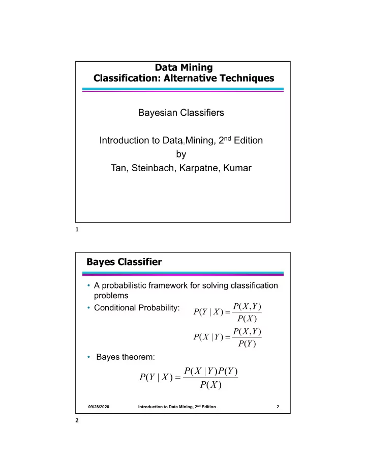
Data Mining Classification: Alternative Techniques Bayesian Classifiers Introduction to Data Mining, 2 nd Edition by Tan, Steinbach, Karpatne, Kumar 1 Bayes Classifier A probabilistic framework for solving classification


  1. Data Mining Classification: Alternative Techniques Bayesian Classifiers Introduction to Data Mining, 2 nd Edition 𝑞 � by Tan, Steinbach, Karpatne, Kumar 1 Bayes Classifier • A probabilistic framework for solving classification problems P ( X , Y ) • Conditional Probability:  P ( Y | X ) P ( X ) P ( X , Y )  P ( X | Y ) P ( Y ) • Bayes theorem: P ( X | Y ) P ( Y )  P ( Y | X ) P ( X ) Introduction to Data Mining, 2 nd Edition 09/28/2020 2 2

  2. Using Bayes Theorem for Classification • Consider each attribute and class label as random variables • Given a record with attributes (X 1 , c c c X 2 ,…, X d ) Tid Refund Marital Taxable Income Evade Status – Goal is to predict class Y 1 Yes Single 125K No – Specifically, we want to find the value of 2 No Married 100K No Y that maximizes P(Y| X 1 , X 2 ,…, X d ) 3 No Single 70K No 4 Yes Married 120K No 5 No Divorced 95K Yes • Can we estimate P(Y| X 1 , X 2 ,…, X d ) 6 No Married 60K No directly from data? 7 Yes Divorced 220K No 8 No Single 85K Yes 9 No Married 75K No 10 No Single 90K Yes 1 0 Introduction to Data Mining, 2 nd Edition 09/28/2020 3 3 Using Bayes Theorem for Classification • Approach: – compute posterior probability P(Y | X 1 , X 2 , …, X d ) using the Bayes theorem P ( X X X | Y ) P ( Y )   P ( Y | X X X ) 1 2 d  1 2 n P ( X X X )  1 2 d – Maximum a-posteriori : Choose Y that maximizes P(Y | X 1 , X 2 , …, X d ) – Equivalent to choosing value of Y that maximizes P(X 1 , X 2 , …, X d |Y) P(Y) • How to estimate P(X 1 , X 2 , …, X d | Y )? Introduction to Data Mining, 2 nd Edition 09/28/2020 4 4

  3. Example Data Given a Test Record:    X ( Refund No, Divorced, Income 120K) c c c Tid Refund Marital Taxable • Can we estimate Income Evade Status P(Evade = Yes | X) and P(Evade = No | X)? 1 Yes Single 125K No 2 No Married 100K No 3 No Single 70K No In the following we will replace 4 Yes Married 120K No 5 No Divorced 95K Yes Evade = Yes by Yes, and 6 No Married 60K No Evade = No by No 7 Yes Divorced 220K No 8 No Single 85K Yes 9 No Married 75K No 10 No Single 90K Yes 0 1 Introduction to Data Mining, 2 nd Edition 09/28/2020 5 5 Example Data Given a Test Record:    X ( Refund No, Divorced, Income 120K) c c c Tid Refund Marital Taxable Income Evade Status 1 Yes Single 125K No 2 No Married 100K No 3 No Single 70K No 4 Yes Married 120K No 5 No Divorced 95K Yes 6 No Married 60K No 7 Yes Divorced 220K No 8 No Single 85K Yes 9 No Married 75K No 10 No Single 90K Yes 0 1 Introduction to Data Mining, 2 nd Edition 09/28/2020 6 6

  4. Conditional Independence • X and Y are conditionally independent given Z if P( X | YZ ) = P( X | Z ) • Example: Arm length and reading skills – Young child has shorter arm length and limited reading skills, compared to adults – If age is fixed, no apparent relationship between arm length and reading skills – Arm length and reading skills are conditionally independent given age Introduction to Data Mining, 2 nd Edition 09/28/2020 7 7 Naïve Bayes Classifier • Assume independence among attributes X i when class is given: – P(X 1 , X 2 , …, X d |Y j ) = P(X 1 | Y j ) P(X 2 | Y j )… P(X d | Y j ) – Now we can estimate P(X i | Y j ) for all X i and Y j combinations from the training data – New point is classified to Y j if P(Y j )  P(X i | Y j ) is maximal. Introduction to Data Mining, 2 nd Edition 09/28/2020 8 8

  5. Naïve Bayes on Example Data Given a Test Record:    X ( Refund No, Divorced, Income 120K) c c c Tid Refund Marital Taxable Income Evade P(X | Yes) = Status 1 Yes Single 125K No P(Refund = No | Yes) x 2 No Married 100K No P(Divorced | Yes) x 3 No Single 70K No P(Income = 120K | Yes) 4 Yes Married 120K No 5 No Divorced 95K Yes 6 No Married 60K No P(X | No) = 7 Yes Divorced 220K No P(Refund = No | No) x 8 No Single 85K Yes 9 No Married 75K No P(Divorced | No) x 10 No Single 90K Yes P(Income = 120K | No) 1 0 Introduction to Data Mining, 2 nd Edition 09/28/2020 9 9 Estimate Probabilities from Data • P(y) = fraction of instances of class y c c c – e.g., P(No) = 7/10, Tid Refund Marital Taxable P(Yes) = 3/10 Evade Status Income 1 Yes Single 125K No • For categorical attributes: 2 No Married 100K No 3 No Single 70K No P(X i =c| y) = n c / n 4 Yes Married 120K No 5 No Divorced 95K Yes – where |X i =c| is number of 6 No Married 60K instances having attribute No value X i =c and belonging to 7 Yes Divorced 220K No class y 8 No Single 85K Yes 9 No Married 75K No – Examples: 10 No Single 90K Yes P(Status=Married|No) = 4/7 10 P(Refund=Yes|Yes)=0 Introduction to Data Mining, 2 nd Edition 09/28/2020 10 10

  6. Estimate Probabilities from Data • For continuous attributes: – Discretization: Partition the range into bins: Replace continuous value with bin value  – Attribute changed from continuous to ordinal – Probability density estimation: Assume attribute follows a normal distribution  Use data to estimate parameters of distribution  (e.g., mean and standard deviation) Once probability distribution is known, use it to  estimate the conditional probability P(X i |Y) Introduction to Data Mining, 2 nd Edition 09/28/2020 11 11 Estimate Probabilities from Data • Normal distribution: Tid Refund Marital Taxable Evade Status Income   2 ( X ) i ij  1 1 Yes Single 125K No 2   2 P ( X | Y ) e ij i j 2 No Married 100K No  2 2 ij 3 No Single 70K No – One for each (X i ,Y i ) pair 4 Yes Married 120K No 5 No Divorced 95K Yes • For (Income, Class=No): 6 No Married 60K No 7 Yes Divorced 220K No – If Class=No 8 No Single 85K Yes  sample mean = 110 9 No Married 75K No  sample variance = 2975 10 No Single 90K Yes 10 1 ( 120  110 ) 2     P ( Income 120 | No ) e 0 . 0072 2 ( 2975 )  2 ( 54 . 54 ) Introduction to Data Mining, 2 nd Edition 09/28/2020 12 12

  7. Example of Naïve Bayes Classifier Given a Test Record:    X ( Refund No, Divorced, Income 120K) Naïve Bayes Classifier: P(Refund = Yes | No) = 3/7 • P(X | No) = P(Refund=No | No) P(Refund = No | No) = 4/7  P(Divorced | No) P(Refund = Yes | Yes) = 0  P(Income=120K | No) P(Refund = No | Yes) = 1 P(Marital Status = Single | No) = 2/7 = 4/7  1/7  0.0072 = 0.0006 P(Marital Status = Divorced | No) = 1/7 P(Marital Status = Married | No) = 4/7 • P(X | Yes) = P(Refund=No | Yes) P(Marital Status = Single | Yes) = 2/3  P(Divorced | Yes) P(Marital Status = Divorced | Yes) = 1/3  P(Income=120K | Yes) P(Marital Status = Married | Yes) = 0 = 1  1/3  1.2  10 -9 = 4  10 -10 For Taxable Income: If class = No: sample mean = 110 Since P(X|No)P(No) > P(X|Yes)P(Yes) sample variance = 2975 If class = Yes: sample mean = 90 Therefore P(No|X) > P(Yes|X) sample variance = 25 => Class = No Introduction to Data Mining, 2 nd Edition 09/28/2020 13 13 Naïve Bayes Classifier can make decisions with partial information about attributes in the test record Even in absence of information P(Yes) = 3/10 about any attributes, we can use Apriori Probabilities of Class P(No) = 7/10 Variable: If we only know that marital status is Divorced, then: Naïve Bayes Classifier: P(Yes | Divorced) = 1/3 x 3/10 / P(Divorced) P(Refund = Yes | No) = 3/7 P(No | Divorced) = 1/7 x 7/10 / P(Divorced) P(Refund = No | No) = 4/7 P(Refund = Yes | Yes) = 0 If we also know that Refund = No, then P(Refund = No | Yes) = 1 P(Marital Status = Single | No) = 2/7 P(Yes | Refund = No, Divorced) = 1 x 1/3 x 3/10 / P(Marital Status = Divorced | No) = 1/7 P(Divorced, Refund = No) P(Marital Status = Married | No) = 4/7 P(No | Refund = No, Divorced) = 4/7 x 1/7 x 7/10 / P(Marital Status = Single | Yes) = 2/3 P(Marital Status = Divorced | Yes) = 1/3 P(Divorced, Refund = No) P(Marital Status = Married | Yes) = 0 If we also know that Taxable Income = 120, then For Taxable Income: P(Yes | Refund = No, Divorced, Income = 120) = 1.2 x10 -9 x 1 x 1/3 x 3/10 / If class = No: sample mean = 110 sample variance = 2975 P(Divorced, Refund = No, Income = 120 ) If class = Yes: sample mean = 90 P(No | Refund = No, Divorced Income = 120) = sample variance = 25 0.0072 x 4/7 x 1/7 x 7/10 / P(Divorced, Refund = No, Income = 120) Introduction to Data Mining, 2 nd Edition 09/28/2020 14 14

Download Presentation
Download Policy: The content available on the website is offered to you 'AS IS' for your personal information and use only. It cannot be commercialized, licensed, or distributed on other websites without prior consent from the author. To download a presentation, simply click this link. If you encounter any difficulties during the download process, it's possible that the publisher has removed the file from their server.

Recommend


More recommend