[PPT] - Overview of Fourier Representation Properties Review of Signal Types PowerPoint Presentation

SLIDE 1

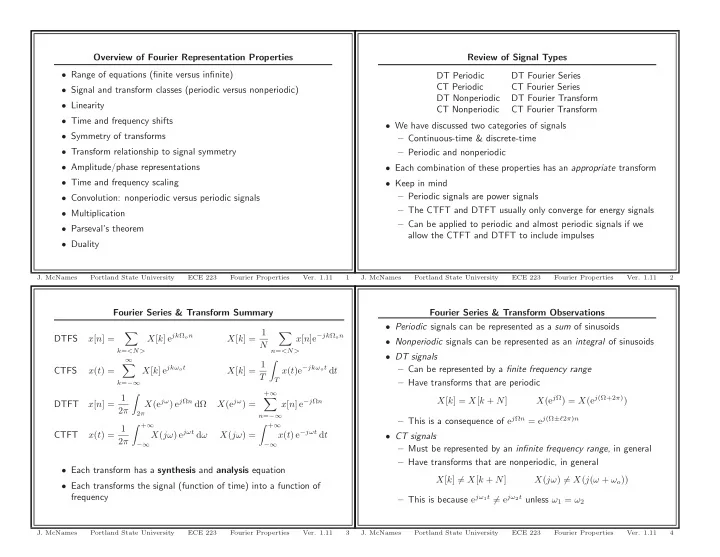
Fourier Series & Transform Summary DTFS x[n] =

k=<N>

X[k] ejkΩon X[k] = 1 N

n=<N>

x[n]e−jkΩon CTFS x(t) =

∞

k=−∞

X[k] ejkωot X[k] = 1 T

T

x(t)e−jkωot dt DTFT x[n] = 1 2π

2π

X(ejω) ejΩn dΩ X(ejω) =

+∞

n=−∞

x[n] e−jΩn CTFT x(t) = 1 2π +∞

−∞

X(jω) ejωt dω X(jω) = +∞

−∞

x(t) e−jωt dt

Each transform has a synthesis and analysis equation
Each transforms the signal (function of time) into a function of

frequency

J. McNames

Portland State University ECE 223 Fourier Properties

Ver. 1.11

3

Overview of Fourier Representation Properties

Range of equations (finite versus infinite)
Signal and transform classes (periodic versus nonperiodic)
Linearity
Time and frequency shifts
Symmetry of transforms
Transform relationship to signal symmetry
Amplitude/phase representations
Time and frequency scaling
Convolution: nonperiodic versus periodic signals
Multiplication
Parseval’s theorem
Duality
J. McNames

Portland State University ECE 223 Fourier Properties

Ver. 1.11

1

Fourier Series & Transform Observations

Periodic signals can be represented as a sum of sinusoids
Nonperiodic signals can be represented as an integral of sinusoids
DT signals

– Can be represented by a finite frequency range – Have transforms that are periodic X[k] = X[k + N] X(ejΩ) = X(ej(Ω+2π)) – This is a consequence of ejΩn = ej(Ω±ℓ2π)n

CT signals

– Must be represented by an infinite frequency range, in general – Have transforms that are nonperiodic, in general X[k] = X[k + N] X(jω) = X(j(ω + ωo)) – This is because ejω1t = ejω2t unless ω1 = ω2

J. McNames

Portland State University ECE 223 Fourier Properties

Ver. 1.11

4

Review of Signal Types DT Periodic DT Fourier Series CT Periodic CT Fourier Series DT Nonperiodic DT Fourier Transform CT Nonperiodic CT Fourier Transform

We have discussed two categories of signals

– Continuous-time & discrete-time – Periodic and nonperiodic

Each combination of these properties has an appropriate transform
Keep in mind

– Periodic signals are power signals – The CTFT and DTFT usually only converge for energy signals – Can be applied to periodic and almost periodic signals if we allow the CTFT and DTFT to include impulses

J. McNames

Portland State University ECE 223 Fourier Properties

Ver. 1.11

2

SLIDE 2

Example 1: Linearity Derive one of the four linearity relationships given on the previous slide.

J. McNames

Portland State University ECE 223 Fourier Properties

Ver. 1.11

7

Notes on Terminology

Many of the transforms share the same properties
The following slides cover the primary properties of the transforms
I will use the word transform generally to refer to both the Fourier

series transforms and the Fourier transforms

The book avoids this and uses the word representation
J. McNames

Portland State University ECE 223 Fourier Properties

Ver. 1.11

5

Application Example 1: Applying the Definition Suppose two people sing into a microphone at the same time. Under what conditions is it possible to design a linear time-invariant filter that separates one of the voices? What characteristics would you want the filter to have?

J. McNames

Portland State University ECE 223 Fourier Properties

Ver. 1.11

8

Property 1: Linearity a1x1[n] + a2x2[n] FS ⇐ ⇒ a1X1[k] + a2X2[k]

FT

⇐ ⇒ a1X1(ejω) + a2X2(ejω) a1x1(t) + a2x2(t) FS ⇐ ⇒ a1X1[k] + a2X2[k]

FT

⇐ ⇒ a1X1(jω) + a2X2(jω)

All of the Fourier transforms are linear
This follows directly from the linearity property of sums and

integrals

Note that for periodic signals, both components must have the

same fundamental period

J. McNames

Portland State University ECE 223 Fourier Properties

Ver. 1.11

6

SLIDE 3

Application Example 2: Workspace

J. McNames

Portland State University ECE 223 Fourier Properties

Ver. 1.11

11

Application Example 1: Workspace

J. McNames

Portland State University ECE 223 Fourier Properties

Ver. 1.11

9

Property 2: Time Shift x[n − no] FS ⇐ ⇒ e−jkΩonoX[k]

FT

⇐ ⇒ e−jΩnoX(ejΩ) x(t − to) FS ⇐ ⇒ e−jkωotoX[k]

FT

⇐ ⇒ e−jωtoX(jω)

What effect does a time shift have on even/odd symmetry in

general?

What effect does a time shift have on phase?
Suppose the phase of the Fourier representation is zero at all
frequencies. What is the effect of shifting the signal?
What effect does a time shift have on amplitude?
J. McNames

Portland State University ECE 223 Fourier Properties

Ver. 1.11

12

Application Example 2: Applying the Definition Suppose you obtain an old recording of a song that you like that is corrupted with a constant humming background noise. Is it possible to design an LTI filter that will eliminate the humm? What characteristics would you want the filter to have? How much would it distort the original signal?

J. McNames

Portland State University ECE 223 Fourier Properties

Ver. 1.11

10

SLIDE 4

Application Example 3: Speaker Recognition Suppose you are asked to design a security system that only allows a single authorized person to open a door. To confirm the person’s identity, they must press a button and speak a password.

How would you design such a system?
How would you account for the variable delay between the start of

the signal (when they push the button) and when they speak the word?

How would you prevent an intruder from entering even if they say

the same password?

J. McNames

Portland State University ECE 223 Fourier Properties

Ver. 1.11

15

Example 2: Time Shift Derive one of the four time-shift relationships on the previous slide.

J. McNames

Portland State University ECE 223 Fourier Properties

Ver. 1.11

13

Application Example 3: Workspace

J. McNames

Portland State University ECE 223 Fourier Properties

Ver. 1.11

16

Example 2: Workspace

J. McNames

Portland State University ECE 223 Fourier Properties

Ver. 1.11

14

SLIDE 5

Example 3: Frequency Shift Derive one of the four frequency-shift relationships on the previous slide.

J. McNames

Portland State University ECE 223 Fourier Properties

Ver. 1.11

19

Application Example 3: Workspace

J. McNames

Portland State University ECE 223 Fourier Properties

Ver. 1.11

17

Example 3: Workspace

J. McNames

Portland State University ECE 223 Fourier Properties

Ver. 1.11

20

Property 3: Frequency Shift ejksΩonx[n]

FS

⇐ ⇒ X[k − ks] ejΩsnx[n]

FT

⇐ ⇒ X(ej(Ω−Ωs)) ejksωotx(t)

FS

⇐ ⇒ X[k − ks] ejωstx(t)

FT

⇐ ⇒ X (j(ω − ωs))

Ωs and ωs is the frequency of the modulating complex sinusoid
For periodic signals the modulating complex sinusoid must be an

integer multiple of the fundamental frequency, ksΩo (why?)

What effect does multiplying (modulating) a signal with a

complex sinusoid have?

J. McNames

Portland State University ECE 223 Fourier Properties

Ver. 1.11

18

SLIDE 6

Example 4: Workspace

J. McNames

Portland State University ECE 223 Fourier Properties

Ver. 1.11

23

Application Example 4: Communications Channel Suppose you wish to transmit a stereo signal over a single telephone

line. You can model a telephone line as a lowpass filter with a 4 kHz

passband.

How can you combine the two signals into a single signal in such a

way that you can extract the original signals?

What must you compromise in combining the two signals into a

single signal?

What properties must the signals have in order to send them over

the telephone line without loss?

J. McNames

Portland State University ECE 223 Fourier Properties

Ver. 1.11

21

Property 4: Transform Symmetry X[−k] = X∗[k] X(e−jΩ) = X∗(ejω) X(−jω) = X∗(jω)

Each transform can be used to synthesize the signal as a sum or

integral of complex sinusoids

The resulting signal is real
Thus all the imaginary components must cancel (sum or integrate

to zero)

This results in the complex-conjugate symmetry of the coefficients
J. McNames

Portland State University ECE 223 Fourier Properties

Ver. 1.11

24

Example 4: Workspace

J. McNames

Portland State University ECE 223 Fourier Properties

Ver. 1.11

22

SLIDE 7

Property 4: Transform Symmetry Continued If the signal is real, then the transforms are complex-conjugate symmetric about the origin X[−k] = X∗[k] X(e−jΩ) = X∗(ejω) X(−jω) = X∗(jω)

This implies

– The real part of the transforms are even – The imaginary part of the transforms are odd – The magnitude is even – The phase is odd

When this symmetry is present, it is only necessary to consider

and plot the transforms for positive frequencies

J. McNames

Portland State University ECE 223 Fourier Properties

Ver. 1.11

27

Example 4: Transform Symmetry Derive one of the four complex-conjugate symmetry relationships listed

n the previous slide given that the signal is real-valued.
J. McNames

Portland State University ECE 223 Fourier Properties

Ver. 1.11

25

Property 5: Transform Relationship to Signal Symmetry xe[n] = 1

2 (x[n] + x[−n])

xe(t) = 1

2 [x(t) + x(−t)]

xo[n] = 1

2 (x[n] − x[−n])

xo(t) = 1

2 [x(t) − x(−t)]

x[n] = xe[n] + xo[n] x(t) = xe(t) + xo(t)

Every signal can be expressed as a sum of even and odd signals
Even signals can be represented as a sum or integral of cosines
Odd signals can be represented as a sum or integral of sines
The real part of the Fourier coefficients represent the coefficients
f the cosines
The imaginary part of the Fourier coefficients represent the

coefficients of the sines

J. McNames

Portland State University ECE 223 Fourier Properties

Ver. 1.11

28

Example 4: Workspace

J. McNames

Portland State University ECE 223 Fourier Properties

Ver. 1.11

26

SLIDE 8

Example 5: Workspace

J. McNames

Portland State University ECE 223 Fourier Properties

Ver. 1.11

31

Property 5: Transform Relationship to Signal Symmetry If the signal is real, then xe[n] FS ⇐ ⇒ Re{X[k]}

FT

⇐ ⇒ Re{X(ejΩ)} xo[n] FS ⇐ ⇒ Im{X[k]}

FT

⇐ ⇒ Im{X(ejΩ)} xe(t) FS ⇐ ⇒ Re{X[k]}

FT

⇐ ⇒ Re{X(jω)} xo(t) FS ⇐ ⇒ Im{X[k]}

FT

⇐ ⇒ Im{X(jω)}

Even signals have Fourier coefficients that are real
Odd signals have Fourier coefficients that are imaginary
Signals without even or odd symmetry are complex
J. McNames

Portland State University ECE 223 Fourier Properties

Ver. 1.11

29

Property 6: Amplitude-Phase Representation If the signal is real, each of the synthesis equations can be written as x[n] =

⌈N/2⌉

k=0

A[k] cos(kΩon + θ[k]) x[n] = 1 π π A(ejΩ) cos

Ωn + θ(ejΩ)
dΩ

x(t) =

∞

k=0

A[k] cos(kωot + θ[k]) x(t) = 1 π ∞ A(jω) cos (ωt + θ(jω)) dω

The magnitude of the Fourier coefficients represents the

magnitude of a combination of cosine and sine at each frequency

Complex phase angle of the coefficients represents the phase of

the combined cosine

J. McNames

Portland State University ECE 223 Fourier Properties

Ver. 1.11

32

Example 5: Transform Relationship to Signal Symmetry Derive one of the eight relationships listed on the previous slide given that the signal is real-valued. Hint: use the complex-conjugate symmetry of the transform.

J. McNames

Portland State University ECE 223 Fourier Properties

Ver. 1.11

30

SLIDE 9

Example 6: Workspace

J. McNames

Portland State University ECE 223 Fourier Properties

Ver. 1.11

35

Example 6: Transform Relationship to Signal Symmetry Derive one of the amplitude-phase forms listed on the previous slide given that the signal is real-valued. Hint: use the complex-conjugate symmetry of the transform.

J. McNames

Portland State University ECE 223 Fourier Properties

Ver. 1.11

33

Amplitude/Phase versus Real/Imaginary Plots

Engineers often plot the Fourier transforms versus frequency as

part of signal analysis

This can lead to insights that guide design
The transforms are complex-valued functions of frequency
Requires two plots to fully represent
Two obvious choices

– Rectangular coordinates: Real and imaginary components versus frequency – Polar coordinates: Amplitude and phase versus frequency

Recall:

– Real component corresponds to even component of signal – Imaginary component corresponds to odd component of signal

But an even/odd signal decomposition, x(t) = xe(t) + xo(t), is

rarely helpful in practice

J. McNames

Portland State University ECE 223 Fourier Properties

Ver. 1.11

36

Example 6: Workspace

J. McNames

Portland State University ECE 223 Fourier Properties

Ver. 1.11

34

SLIDE 10

Application Example 5: Polar versus Rectangular

500 1000 1500 2000 2500 3000 3500 4000 4500 5000 5500 −10 −5 5 10 15 Real FT 500 1000 1500 2000 2500 3000 3500 4000 4500 5000 5500 −10 10 20 Frequency (Hz) Imaginary FT

J. McNames

Portland State University ECE 223 Fourier Properties

Ver. 1.11

39

Application Example 5: Polar versus Rectangular Use the fast Fourier transform to estimate the CTFT over a range of frequencies from 0 to half the sampling rate, fs/2, of a 60 ms segment

f speech.
What insights do you gain from studying the FT plots that you

did not gain from studying a time-domain plot?

What type of properties would a communications channel require

to transmit this signal?

What insights do you gain from studying the real, imaginary,

amplitude, and phase plots.

J. McNames

Portland State University ECE 223 Fourier Properties

Ver. 1.11

37

Application Example 5: Polar versus Rectangular

500 1000 1500 2000 2500 3000 3500 4000 4500 5000 5500 5 10 15 20 FT Magnitude 500 1000 1500 2000 2500 3000 3500 4000 4500 5000 5500 −200 −100 100 200 Frequency (Hz) FT Complex Phase (degrees)

J. McNames

Portland State University ECE 223 Fourier Properties

Ver. 1.11

40

Application Example 5: Polar versus Rectangular

1.6 1.61 1.62 1.63 1.64 1.65 −0.25 −0.2 −0.15 −0.1 −0.05 0.05 0.1 0.15 0.2 Time (sec) Linus: Philosophy of Wet Suckers

J. McNames

Portland State University ECE 223 Fourier Properties

Ver. 1.11

38

SLIDE 11

box off; ylabel(’FT Complex Phase (degrees)’); xlabel(’Frequency (Hz)’); AxisSet(6); print -depsc SpeechFTPolar;

J. McNames

Portland State University ECE 223 Fourier Properties

Ver. 1.11

43

Application Example 5: MATLAB Code

function [] = Speech(); close all; [x,fs,nbits] = wavread(’WetSuck.wav’); k = round(fs*1.6):round(fs*1.66); % Look at only 0.5 s x = x(k); nx = length(x); figure; FigureSet(1,’LTX’); t = (k-1)/fs; h = plot(t,x,’b’); set(h,’LineWidth’,0.6); xrng = max(x)-min(x); xlim([min(t) max(t)]); ylim([min(x)-0.01*xrng max(x)+0.01*xrng]); AxisLines; xlabel(’Time (sec)’); ylabel(’’); title(’Linus: Philosophy of Wet Suckers’); box off; AxisSet(8); print -depsc Speech; X = fft(x,2^(max([12,nextpow2(nx)]))); nX = length(X); k = 1:floor((length(X)+1)/2); f = (k-1)*(fs)./(nX+1); figure; FigureSet(1,’LTX’); subplot(2,1,1); h = plot(f,real(X(k)),’r’);

J. McNames

Portland State University ECE 223 Fourier Properties

Ver. 1.11

41

Amplitude/Phase versus Real/Imaginary Plots Continued

The most useful plot is amplitude (or squared amplitude) of the

transform versus frequency

Only need to plot transform for positive frequencies (why?)
Examining the phase is rarely useful for signal analysis

– Phase is sensitive to time-shift of signal – Phase is bounded: −π ≤ θ ≤ π

Phase is important for system analysis

– Consider bode plots – Linearity of phase is an important consideration – More on this later

J. McNames

Portland State University ECE 223 Fourier Properties

Ver. 1.11

44

set(h,’LineWidth’,0.6); xlim([min(f) max(f)]); ylim([1.05*min(real(X(k))) 1.05*max(real(X(k)))]); set(gca,’XTick’,[0:500:max(f)]); AxisLines; box off; ylabel(’Real FT’); subplot(2,1,2); h = plot(f,imag(X(k)),’r’); set(h,’LineWidth’,0.6); xlim([min(f) max(f)]); ylim([1.05*min(imag(X(k))) 1.05*max(imag(X(k)))]); set(gca,’XTick’,[0:500:max(f)]); AxisLines; box off; ylabel(’Imaginary FT’); xlabel(’Frequency (Hz)’); AxisSet(6); print -depsc SpeechFTRectangular; figure; FigureSet(1,’LTX’); subplot(2,1,1); h = plot(f,abs(X(k)),’r’); set(h,’LineWidth’,0.6); xlim([min(f) max(f)]); ylim([0 1.05*max(abs(X(k)))]); set(gca,’XTick’,[0:500:max(f)]); box off; ylabel(’FT Magnitude’); subplot(2,1,2); h = plot(f,angle(X(k))*180/pi,’r’); set(h,’LineWidth’,0.6); xlim([min(f) max(f)]); ylim([-200 200]); set(gca,’XTick’,[0:500:max(f)]); AxisLines;

J. McNames

Portland State University ECE 223 Fourier Properties

Ver. 1.11

42

SLIDE 12

Example 7: Workspace

J. McNames

Portland State University ECE 223 Fourier Properties

Ver. 1.11

47

Property 7: Convolution of Nonperiodic Signals x[n] ∗ h[n] =

∞

k=−∞

h[k]x[n − k] =

∞

k=−∞

x[k]h[n − k] x(t) ∗ h(t) = ∞

−∞

h(τ)x(t − τ) dτ = ∞

−∞

x(τ)h(t − τ) dτ

Convolution is defined differently for periodic and nonperiodic

signals

We will discuss convolution for nonperiodic signals first
This is the convolution you are already familiar with
J. McNames

Portland State University ECE 223 Fourier Properties

Ver. 1.11

45

Property 7: Convolution Concepts x[n] ∗ h[n]

FT

⇐ ⇒ X(ejω)H(ejω) x(t) ∗ h(t)

FT

⇐ ⇒ X(jω)H(jω)

This is very similar to what we used the Laplace transform for
Key differences

– Can be applied to two-sided signals – Cannot be applied to signals with infinite energy – Works in discrete-time as well as continuous-time

Enables us to think of a system in terms of how it scales and

shifts the complex phase angle of each complex sinusoid component of the signal

This is very useful if we have a good notion of which components

are present in a signal via the Fourier transform

J. McNames

Portland State University ECE 223 Fourier Properties

Ver. 1.11

48

Example 7: Nonperiodic Continuous-Time Derive either the DT or CT relationship between the convolution of two signals and their transforms x(t) ∗ h(t)

FT

⇐ ⇒ X(jω)H(jω)

r

x[n] ∗ h[n]

FT

⇐ ⇒ X(ejω)H(ejω)

J. McNames

Portland State University ECE 223 Fourier Properties

Ver. 1.11

46

SLIDE 13

Example 8: Workspace

J. McNames

Portland State University ECE 223 Fourier Properties

Ver. 1.11

51

Property 8: Convolution of Periodic Signals x(t) ⊛ z(t) =

<T >

x(τ)z(t − τ) dτ x(t) ⊛ z(t)

FS

⇐ ⇒ TX[k]Z[k] x[n] ⊛ z[n] =

k=<N>

x[k]z[n − k] x[n] ⊛ z[n]

FS

⇐ ⇒ NX[k]Z[k]

Convolution of periodic signals occurs in signal analysis, but not

system analysis

This is because stable systems do not have impulse responses that

are periodic

Nonetheless, convolution is useful for signal analysis
J. McNames

Portland State University ECE 223 Fourier Properties

Ver. 1.11

49

Property 9: Differentiation and Integration

These are listed in the book (Table 3.6)
They are very similar to the corresponding Laplace transform

properties

In most cases, these are handled with other transforms

– Differential equations are usually handled with the Laplace transform – Difference equations are handled with the z transform

J. McNames

Portland State University ECE 223 Fourier Properties

Ver. 1.11

52

Example 8: Convolution of Periodic Signals Derive either the DT or CT relationship between the convolution of two signals and their transforms x(t) ⊛ h(t)

FS

⇐ ⇒ TX[k]Z[k] x[n] ⊛ h[n]

FS

⇐ ⇒ NX[k]Z[k]

J. McNames

Portland State University ECE 223 Fourier Properties

Ver. 1.11

50

SLIDE 14

Example 9: Workspace

J. McNames

Portland State University ECE 223 Fourier Properties

Ver. 1.11

55

Property 10: Signal Multiplication x[n] z[n]

FS

⇐ ⇒ X[k] ⊛ Z[k] x[n] z[n]

FT

⇐ ⇒ 1 2π X(ejω) ⊛ Z(ejω) x(t) z(t)

FS

⇐ ⇒ X[k] ∗ Z[k] x(t) z(t)

FT

⇐ ⇒ 1 2π X(jω) ∗ Z(jω)

Recall that convolution in the time domain is equivalent to

multiplication in the frequency domain

This shows that multiplication in the time domain is equivalent to

convolution in the frequency domain

Recall that the DT transforms are periodic and the CT transforms

are non periodic

Naturally, it works out that the DT transforms have circular

convolution and the CT transforms have ordinary convolution

J. McNames

Portland State University ECE 223 Fourier Properties

Ver. 1.11

53

Windowing xs(t) = wT (t)x(t) =

wT (t)x(t)

|t| ≤ T |t| > T Xs(jω) = T

−T

wT (t)x(t)e−jωt dt

To estimate the Fourier transform of a signal, modern equipment

uses digital signal processing (DSP)

This essentially means the signal is first sampled, and then

processed

Only a finite segment of the sample can be analyzed, xs(t)
Using this segment can be modelled as multiplying the original

signal with a finite-duration window, w(t)

This processing step is called windowing
How does this affect the estimated spectrum of the signal?
J. McNames

Portland State University ECE 223 Fourier Properties

Ver. 1.11

56

Example 9: Signal Multiplication Derive one of the four relationships on the previous slide.

J. McNames

Portland State University ECE 223 Fourier Properties

Ver. 1.11

54

SLIDE 15

Example 10: Workspace Hint: we found the Fourier transform of a pulse earlier: p(t) = u(t + T) − u(t − T) =

1

|t| < T |t| > T P(jω) = 2T sin(ωT) ωT = 2T sinc ωT π

J. McNames

Portland State University ECE 223 Fourier Properties

Ver. 1.11

59

Windowing Continued

t x(t) t w(t) t w(t) x(t)

ω ω ω |X(jω)| |W (jω)|

1 2π |X(jω) ∗ W (jω)|

Since only of a segment of the signal is available, the Fourier

transform of the signal cannot be calculated exactly

Windowing is necessary to estimate the spectrum from a segment
f the signal with finite duration
In the frequency domain, this filters or blurs the spectrum
J. McNames

Portland State University ECE 223 Fourier Properties

Ver. 1.11

57

Example 10: Window and Windowed Segment

−5 −4 −3 −2 −1 1 2 3 4 5 −1 −0.5 0.5 1 Window fo= 10.0 Hz T=0.100 s Window w(t) −5 −4 −3 −2 −1 1 2 3 4 5 −1 −0.5 0.5 1 Time (s) Windowed Signal y(t) = w(t) xs(t)

J. McNames

Portland State University ECE 223 Fourier Properties

Ver. 1.11

60

Example 5: Windowing Your oscilloscopes in the lab must estimate the CT Fourier transform

f a signal using a finite segment of the data. Calculate and plot the

CT Fourier transform of a windowed sinusoid with a fundamental frequency of f0 = 10 Hz for a range of window lengths. Select the sinusoidal phase and window alignment such that the signal has even symmetry (why?).

How does the estimated spectrum compare to the true spectrum?
What happens as the window length decreases towards zero?
What happens as the window length increases towards infinity?
What would the transform of an ideal window be?
What are the disadvantages of using a rectangular window,

w(t) = pT (t)?

J. McNames

Portland State University ECE 223 Fourier Properties

Ver. 1.11

58

SLIDE 16

Example 10: Window and Windowed Segment Transforms

−15 −10 −5 5 10 15 5 10 W(jω) Pulse Spectral Amplitude fo= 10.0 Hz T=0.500 s −15 −10 −5 5 10 15 2 4 Y(jω) Frequency (rad/s)

J. McNames

Portland State University ECE 223 Fourier Properties

Ver. 1.11

63

Example 10: Window and Windowed Segment Transforms

−15 −10 −5 5 10 15 5 10 W(jω) Pulse Spectral Amplitude fo= 10.0 Hz T=0.100 s −15 −10 −5 5 10 15 2 4 Y(jω) Frequency (rad/s)

J. McNames

Portland State University ECE 223 Fourier Properties

Ver. 1.11

61

Example 10: Window and Windowed Segment

−5 −4 −3 −2 −1 1 2 3 4 5 −1 −0.5 0.5 1 Window fo= 10.0 Hz T=1.000 s Window w(t) −5 −4 −3 −2 −1 1 2 3 4 5 −1 −0.5 0.5 1 Time (s) Windowed Signal y(t) = w(t) xs(t)

J. McNames

Portland State University ECE 223 Fourier Properties

Ver. 1.11

64

Example 10: Window and Windowed Segment

−5 −4 −3 −2 −1 1 2 3 4 5 −1 −0.5 0.5 1 Window fo= 10.0 Hz T=0.500 s Window w(t) −5 −4 −3 −2 −1 1 2 3 4 5 −1 −0.5 0.5 1 Time (s) Windowed Signal y(t) = w(t) xs(t)

J. McNames

Portland State University ECE 223 Fourier Properties

Ver. 1.11

62

SLIDE 17

Example 10: Window and Windowed Segment Transforms

−15 −10 −5 5 10 15 5 10 W(jω) Pulse Spectral Amplitude fo= 10.0 Hz T=2.000 s −15 −10 −5 5 10 15 2 4 Y(jω) Frequency (rad/s)

J. McNames

Portland State University ECE 223 Fourier Properties

Ver. 1.11

67

Example 10: Window and Windowed Segment Transforms

−15 −10 −5 5 10 15 5 10 W(jω) Pulse Spectral Amplitude fo= 10.0 Hz T=1.000 s −15 −10 −5 5 10 15 2 4 Y(jω) Frequency (rad/s)

J. McNames

Portland State University ECE 223 Fourier Properties

Ver. 1.11

65

Example 10: Window and Windowed Segment

−5 −4 −3 −2 −1 1 2 3 4 5 −1 −0.5 0.5 1 Window fo= 10.0 Hz T=5.000 s Window w(t) −5 −4 −3 −2 −1 1 2 3 4 5 −1 −0.5 0.5 1 Time (s) Windowed Signal y(t) = w(t) xs(t)

J. McNames

Portland State University ECE 223 Fourier Properties

Ver. 1.11

68

Example 10: Window and Windowed Segment

−5 −4 −3 −2 −1 1 2 3 4 5 −1 −0.5 0.5 1 Window fo= 10.0 Hz T=2.000 s Window w(t) −5 −4 −3 −2 −1 1 2 3 4 5 −1 −0.5 0.5 1 Time (s) Windowed Signal y(t) = w(t) xs(t)

J. McNames

Portland State University ECE 223 Fourier Properties

Ver. 1.11

66

SLIDE 18

Example 10: MATLAB Code Continued

J. McNames

Portland State University ECE 223 Fourier Properties

Ver. 1.11

71

Example 10: Window and Windowed Segment Transforms

−15 −10 −5 5 10 15 5 10 W(jω) Pulse Spectral Amplitude fo= 10.0 Hz T=5.000 s −15 −10 −5 5 10 15 2 4 Y(jω) Frequency (rad/s)

J. McNames

Portland State University ECE 223 Fourier Properties

Ver. 1.11

69

Property 11: Time & Frequency Scaling x[an]

FT

⇐ ⇒ X(ejΩ/a) x(at)

FS

⇐ ⇒ X[k] x(at)

FT

⇐ ⇒ 1 |a|X jω a

Scaling a signal in time inversely scales the spectrum by the same

factor

Scaling a periodic signal shifts the spacing of the harmonic

components, but the amplitudes are the same!

In the DT case, a must be an integer (the signal is not defined at

non-integer samples)

This is equivalent to sampling only 1 out of every a values of x[n]
DT periodic signals are tricky because the fundamental period of

x[an] depends on how a and N are related

J. McNames

Portland State University ECE 223 Fourier Properties

Ver. 1.11

72

Example 10: MATLAB Code

J. McNames

Portland State University ECE 223 Fourier Properties

Ver. 1.11

70

SLIDE 19

Property 12: Parseval’s Theorem DTFS 1 N

n=<N>

|x[n]|2 =

k=<N>

|X[k]|2 DTFT

∞

n=−∞

|x[n]|2 = 1 2π

<2π>
X(ejω)
2 dΩ

CTFS 1 T

<T >

|x(t)|2 dt =

∞

k=−∞

|X[k]|2 CTFT ∞

−∞

|x(t)|2 dt = 1 2π ∞

−∞

|X(jω)|2 dω

The energy/power of the time domain signal is equal to the

energy/power of the frequency domain transform!

J. McNames

Portland State University ECE 223 Fourier Properties

Ver. 1.11

75

Example 11: Time & Frequency Scaling Derive one of the transform relationships on the previous slide.

J. McNames

Portland State University ECE 223 Fourier Properties

Ver. 1.11

73

Example 12: Parseval’s Theorem Derive one of the four relationships on the previous slide.

J. McNames

Portland State University ECE 223 Fourier Properties

Ver. 1.11

76

Example 11: Workspace

J. McNames

Portland State University ECE 223 Fourier Properties

Ver. 1.11

74

SLIDE 20

Application Example 6: Parseval’s Theorem Suppose you wish to transmit a speech signal through a channel with as little bandwidth as possible.

What bandwidth is necessary if you wish to retain 95% of the

signal energy?

Which frequency range should you transmit?
J. McNames

Portland State University ECE 223 Fourier Properties

Ver. 1.11

79

Example 12: Workspace

J. McNames

Portland State University ECE 223 Fourier Properties

Ver. 1.11

77

Application Example 6: Parseval’s Theorem

1.6 1.61 1.62 1.63 1.64 1.65 1.66 1.67 1.68 1.69 −0.25 −0.2 −0.15 −0.1 −0.05 0.05 0.1 0.15 0.2 Time (sec) Linus: Philosophy of Wet Suckers

J. McNames

Portland State University ECE 223 Fourier Properties

Ver. 1.11

80

Property 12: Parseval’s Theorem Comments

Thus the magnitude of the spectrum squared is called

– The energy spectral density for energy (nonperiodic) signals – The power spectral density for power (periodic) signals

This is why the squared magnitude is often plotted versus

frequency instead of just the magnitude

This enables us to talk about what fraction of signal energy is

contained within certain frequency ranges

J. McNames

Portland State University ECE 223 Fourier Properties

Ver. 1.11

78

SLIDE 21

Application Example 6: MATLAB Code Continued

J. McNames

Portland State University ECE 223 Fourier Properties

Ver. 1.11

83

Application Example 6: Parseval’s Theorem

500 1000 1500 2000 2500 3000 3500 4000 4500 5000 5500 100 200 300 400 PSD 500 1000 1500 2000 2500 3000 3500 4000 4500 5000 5500 10 20 30 40 50 60 70 80 90 100 Frequency (Hz) Net Spectral Energy (%)

J. McNames

Portland State University ECE 223 Fourier Properties

Ver. 1.11

81

Property 13: Duality x(t)

FT

⇐ ⇒ X(jω) X(jt)

FT

⇐ ⇒ 2πx(−t) x[n]

FS

⇐ ⇒ X[k] X[n]

FS

⇐ ⇒ 1 N x[−k]

We have already seen many times there are equivalent

relationships between the time and frequency domain x(t − to)

FT

⇐ ⇒ e−jωtoX(jω) ejωotx(t)

FT

⇐ ⇒ X (j(ω − ωo)) δ(t)

FT

⇐ ⇒ 1 1

FT

⇐ ⇒ 2πδ(ω) pT (t)

FT

⇐ ⇒ 2T sinc( ωT

π )

2W sinc( tW

π ) FT

⇐ ⇒ 2π pW (ω)

This occurs due to the similarity of the synthesis and analysis

equations for the CTFT and DTFS

J. McNames

Portland State University ECE 223 Fourier Properties

Ver. 1.11

84

Application Example 6: MATLAB Code

J. McNames

Portland State University ECE 223 Fourier Properties

Ver. 1.11

82

SLIDE 22

Property 13: Duality Comments x(t)

FT

⇐ ⇒ X(jω) X(jt)

FT

⇐ ⇒ 2πx(−t) x[n]

FS

⇐ ⇒ X[k] X[n]

FS

⇐ ⇒ 1 N x[−k]

It occurs for only these two transforms because only these two

have a signal and transform in the same signal class – CTFT: signal and transform are continuous and nonperiodic – DTFS: signal and transform or discrete and periodic

There is also a duality relationship between the DTFT and the

CTFS (see text for details), but this is less important

Duality is useful primarily for calculating transforms
J. McNames

Portland State University ECE 223 Fourier Properties

Ver. 1.11

87

Example 13: Duality Derive one of the four relationships on the previous slide.

J. McNames

Portland State University ECE 223 Fourier Properties

Ver. 1.11

85

Fourier Properties Summary

All four Fourier transforms share most properties
These properties are useful for

– Gaining insight that helps us understand how to interpret the transforms of signals (e.g. Parseval’s theorem) – Gives us tools and ideas for designing systems (e.g. modulation)

J. McNames

Portland State University ECE 223 Fourier Properties

Ver. 1.11

88

Example 13: Workspace

J. McNames

Portland State University ECE 223 Fourier Properties

Ver. 1.11