Overview Grammars A grammar is a 4-tuple ( N, , S, P ) where - - PowerPoint PPT Presentation

Towards more complex grammar systems Some basic formal language theory

Detmar Meurers: Intro to Computational Linguistics I OSU, LING 684.01

Overview

• Grammars, or: how to specify linguistic knowledge
• Automata, or: how to process with linguistic knowledge
• Levels of complexity in grammars and automata:

The Chomsky hierarchy

Grammars

A grammar is a 4-tuple (N, Σ, S, P) where

• N is a finite set of non-terminals
• Σ is a finite set of terminal symbols,

with N ∩ Σ = ∅

• S is a distinguished start symbol, with S ∈ N
• P is a finite set of rewrite rules of the form α → β, with α, β ∈

(N ∪ Σ)∗ and α including at least one non-terminal symbol.

A simple example

N = {S, NP , VP , Vi, Vt, Vs} Σ = {John, Mary, laughs, loves, thinks} S = S P =                S → NP VP VP → Vi VP → Vt NP VP → Vs S NP → John NP → Mary Vi → laughs Vt → loves Vs → thinks               

How does a grammar define a language?

Assume α, β ∈ (N ∪ Σ)∗, with α containing at least one non-terminal.

• A sentential form for a grammar G is defined as:

− The start symbol S of G is a sentential form. − If αβγ is a sentential form and there is a rewrite rule β → δ then αδγ is a sentential form.

• α (directly or immediately) derives β if α → β ∈ P. One writes:

− α ⇒∗ β if β is derived from α in zero or more steps − α ⇒+ β if β is derived from α in one or more steps

• A sentence is a sentential form consisting only of terminal symbols.
• The language L(G) generated by the grammar G is the set of all

sentences which can be derived from the start symbol S, i.e., L(G) = {γ|S ⇒∗ γ}

Processing with grammars: automata

An automaton in general has three components:

• an input tape, divided into squares with a read-write head positioned
• ver one of the squares
• an auxiliary memory characterized by two functions

− fetch: memory configuration → symbols − store: memory configuration × symbol → memory configuration

• and a finite-state control relating the two components.

Different levels of complexity in grammars and automata

Let A, B ∈ N, x ∈ Σ, α, β, γ ∈ (Σ ∪ T)∗, and δ ∈ (Σ ∪ T)+, then: Type Automaton Grammar Memory Name Rule Name Unbounded TM α → β General rewrite 1 Bounded LBA β A γ → β δ γ Context-sensitive 2 Stack PDA A → β Context-free 3 None FSA A → xB, A → x Right linear Abbreviations: – TM: Turing Machine – LBA: Linear-Bounded Automaton – PDA: Push-Down Automaton – FSA: Finite-State Automaton

Type 3: Right-Linear Grammars and FSAs

A right-linear grammar is a 4-tuple (N, Σ, S, P) with P a finite set of rewrite rules of the form α → β, with α ∈ N and β ∈ {γδ|γ ∈ Σ∗, δ ∈ N ∪ {ǫ}}, i.e.: − left-hand side of rule: a single non-terminal, and − right-hand side of rule: a string containing at most one non-terminal, as the rightmost symbol Right-linear grammars are formally equivalent to left-linear grammars. A finite-state automaton consists of – a tape – a finite-state control – no auxiliary memory

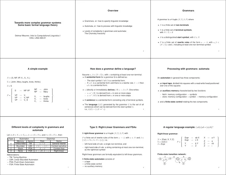
A regular language example: (ab|c)ab ∗ (a|cb)?

Right-linear grammar: N = {Expr, X, Y, Z} Σ = {a,b,c} S = Expr P =          Expr → ab X Expr → c X Y → b Y Y → Z X → a Y Z → a Z → cb Z → ǫ          Finite-state transition network: 1 2 3 4 5 b c a a c b a b

Thinking about regular languages

− A language is regular iff one can define a FSM (or regular expression) for it. − An FSM only has a fixed amount of memory, namely the number of states. − Strings longer than the number of states, in particular also any infinite

• nes, must result from a loop in the FSM.

− Pumping Lemma: if for an infinite string there is no such loop, the string cannot be part of a regular language.

Type 2: Context-Free Grammars and Push-Down Automata

A context-free grammar is a 4-tuple (N, Σ, S, P) with P a finite set of rewrite rules of the form α → β, with α ∈ N and β ∈ (Σ ∪ N)∗, i.e.: − left-hand side of rule: a single non-terminal, and − right-hand side of rule: a string of terminals and/or non-terminals A push-down automaton is a − finite state automaton, with a − stack as auxiliary memory

A context-free language example: anbn

Context-free grammar: N = {S} Σ = {a, b} S = S P =

• S

→ a S b S → ǫ

• Push-down automaton:

a + push x b + pop x 1 ǫ

Type 1: Context-Sensitive Grammars and Linear-Bounded Automata

A rule of a context-sensitive grammar – rewrites at most one non-terminal from the left-hand side. – right-hand side of a rule required to be at least as long as the left- hand side, i.e. only contains rules of the form α → β with |α| ≤ |β| and optionally S → ǫ with the start symbol S not occurring in any β. A linear-bounded automaton is a – finite state automaton, with an – auxiliary memory which cannot exceed the length of the input string.

A context-sensitive language example: anbncn

Context-sensitive grammar: N = {S, B, C} Σ = {a, b} S = S P =                S → a S B C, S → a b C, b B → b b, b C → b c, c C → c c, C B → B C               

Type 0: General Rewrite Grammar and Turing Machines

• In a general rewrite grammar there are no restrictions on the form
• f a rewrite rule.
• A turing machine has an unbounded auxiliary memory.
• Any language for which there is a recognition procedure can be

defined, but recognition problem is not decidable.

Properties of different language classes

Languages are sets of strings, so that one can apply set operations to languages and investigate the results for particular language classes. Some closure properties: − All language classes are closed under union with themselves. − All language classes are closed under intersection with regular languages. − The class of context-free languages is not closed under intersection with itself. Proof: The intersection of the two context-free languages L1 and L2 is not context free: − L1 =

• anbnci|n ≥ 1 and i ≥ 0
• − L2 =
• ajbncn|n ≥ 1 and j ≥ 0
• − L1 ∩ L2 = {anbncn|n ≥ 1}

Criteria under which to evaluate grammar formalisms

There are three kinds of criteria: – linguistic naturalness – mathematical power – computational effectiveness and efficiency The weaker the type of grammar: – the stronger the claim made about possible languages – the greater the potential efficiency of the parsing procedure Reasons for choosing a stronger grammar class: – to capture the empirical reality of actual languages – to provide for elegant analyses capturing more generalizations (→ more “compact” grammars)

Language classes and natural languages

Natural languages are not regular (1) a. The mouse escaped.

• b. The mouse that the cat chased escaped.
• c. The mouse that the cat that the dog saw chased escaped.

d. . . . (2) a. aa

• b. abba
• c. abccba

d. . . . Center-embedding of arbitrary depth needs to be captured to capture language competence → Not possible with a finite state automaton.

Language classes and natural languages (cont.)

• Any finite language is a regular language.
• The argument that natural languages are not regular relies on

competence as an idealization, not performance.

• Note that even if English were regular, a context-free grammar

characterization could be preferable on the grounds that it is more transparent than one using only finite-state methods.

Accounting for the facts

• vs. linguistically sensible analyses

Looking at grammars from a linguistic perspective, one can distinguish their − weak generative capacity, considering only the set of strings generated by a grammar − strong generative capacity, considering the set of strings and their syntactic analyses generated by a grammar Two grammars can be strongly or weakly equivalent.

Example for weakly equivalent grammars

Example string: if x then if y then a else b Grammar 1:                S → if T then S else S, S → if T then S, S → a S → b T → x T → y               

First analysis: if x T then if y T then a S S else b S S Second analysis: if x T then if y T then a S else b S S S

Grammar 2 rules: A weekly equivalent grammar eliminating the ambiguity (only licenses second structure).                            S1 → if T then S1, S1 → if T then S2 else S1, S1 → a, S1 → b, S2 → if T then S2 else S2, S2 → a S2 → b T → x T → y                           

Reading assignment

• Chapter 2 “Basic Formal Language Theory” of our Lecture Notes
• Chapter 3 “Formal Languages and Natural Languages” of our

Lecture Notes

• Chapter 13 “Language and complexity” of Jurafsky and Martin (2000)