Overview Bayesian Model Selection Bayesian Learning of CPTs - PowerPoint PPT Presentation

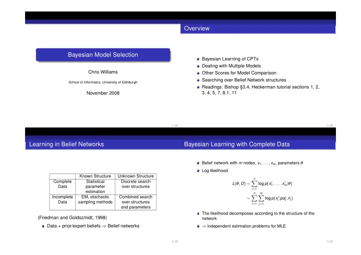
Overview Bayesian Model Selection Bayesian Learning of CPTs Dealing with Multiple Models Chris Williams Other Scores for Model Comparison Searching over Belief Network structures School of Informatics, University of Edinburgh Readings: Bishop §3.4, Heckerman tutorial sections 1, 2, 3, 4, 5, 7, 8.1, 11 November 2008 1 / 22 2 / 22 Learning in Belief Networks Bayesian Learning with Complete Data Belief network with m nodes, x 1 , . . . , x m , parameters θ Log likelihood Known Structure Unknown Structure n Complete Statistical Discrete search � log p ( x i 1 , . . . , x i L ( θ ; D ) = m | θ ) Data parameter over structures i = 1 estimation n m Incomplete EM, stochastic Combined search � � log p ( x i j | pa i = j , θ j ) Data sampling methods over structures i = 1 j = 1 and parameters The likelihood decomposes according to the structure of the (Friedman and Goldszmidt, 1998) network Data + prior/expert beliefs ⇒ Belief networks ⇒ independent estimation problems for MLE 3 / 22 4 / 22

Example: X → Y If priors for each CPT are independent, so are posteriors Posterior for each multinomial CPT P ( X j | Pa j ) is Dirichlet with parameters X Y α ( X j = 1 | pa j ) + n ( X j = 1 | pa j ) , . . . , , α ( X j = r | pa j ) + n ( X j = r | pa j ) Parameters θ X , θ Y | X 5 / 22 6 / 22 Dealing with Multiple Models θ θ X Y|X Let M index possible model structures, with associated parameters θ M x y 1 1 p ( M | D ) ∝ p ( D | M ) p ( M ) x y For complete data (plus some other assumptions) the marginal 2 2 . . likelihood p ( D | M ) can be computed in closed form . . Making predictions x y n n � p ( x n + 1 | D ) = p ( M | D ) p ( x n + 1 | M , D ) Read off from network: complete data = ⇒ posteriors for M � θ X and θ Y | X are independent � = p ( M | D ) p ( x n + 1 | θ M , M ) p ( θ M | D , M ) d θ M Reduces to 3 separate thumbtack-learning problems M Can approximate � M by keeping the best or the top few models 7 / 22 8 / 22

Comparing models Computing P ( D | M ) Bayes factor = P ( D | M 1 ) P ( D | M 2 ) • For the thumbtack example P ( M 1 | D ) P ( M 2 | D ) = P ( M 1 ) P ( M 2 ) . P ( D | M 1 ) r Γ( α ) Γ( α i + n i ) � p ( D | M ) = P ( D | M 2 ) Γ( α + n ) Γ( α i ) Posterior ratio = Prior ratio × Bayes factor i = 1 Strength of evidence from Bayes factor (Kass, 1995; after Jeffreys, Y corresponds to 3 separate thumbtack X • The graph 1961) problems for X , Y | X = heads and Y | X = tails 1 to 3 Not worth more than a bare mention 3 to 20 Positive 20 to 150 Strong > 150 Very strong 9 / 22 10 / 22 General form of P ( D | M ) for a discrete belief network Computation of Marginal Likelihood q i r i m Γ( α ij ) Γ( α ijk + n ijk ) � � � p ( D | M ) = Γ( α ij + n ij ) Γ( α ijk ) i = 1 j = 1 k = 1 where Efficient closed form if i and Pa i = pa j n ijk is the number of cases where X i = x k i No missing data or hidden variables r i is the number of states of X i Parameters are independent in prior q i is the number of configurations of the parents of X i Local distributions are in the exponential family (e.g. multinomial, Gaussian, Poisson, ...) r i r i � � α ij = n ij = n ijk α ijk Conjugate priors are used k = 1 k = 1 Formula due to Cooper and Herskovits (1992) Simply the product of the thumbtack result over all nodes and states of the parents 11 / 22 12 / 22

Example How Bayesian model comparison works Given data D , compare the two models Consider three models M 1 , M 2 and M 3 which are under complex, just right and over complex for a particular dataset D ∗ X Y model 1 Note that P ( D | M i ) must be normalized * X Y D model 2 P(D|M ) 1 Counts: hh = 6, ht = 2, th = 8, tt = 4, from marginal probabilities P(D|M ) 2 P ( X = h ) = 0 . 4 and P ( Y = h ) = 0 . 7 P(D|M ) 3 Bayes factor = P ( D | M 1 ) P ( D | M 2 ) = 1 . 97 in favour of model 1 Log Likelihood criterion favours model 2 Warning: it can make sense to use a model with an infinite log L ( M 1 ) − log L ( M 2 ) = − 0 . 08 number of parameters (but in a way that the prior is “nice”) 13 / 22 14 / 22 Other scores for comparing models ∆ Above we have used P ( D | M ) to score models. Other ideas include θ * Maximum likelihood ∆ 0 Another view (for a single parameter θ ) L ( M ; D ) = max θ M L ( θ M , M ; D ) � P ( D | M i ) = p ( D | θ, M i ) p ( θ | M i ) d θ Bad choice: adding arcs always helps p ( D | θ ∗ , M i ) p ( θ ∗ | M i )∆ ≃ Example from supervised learning p ( D | θ ∗ , M i ) ∆ ≃ 1 1 1 linear regression cubic regression 9th−order regression sin(2 π x) sin(2 π x) sin(2 π x) ∆ 0 0.8 data 0.8 data 0.8 data 0.6 0.6 0.6 0.4 0.4 0.4 This last term is known as an Occam factor 0.2 0.2 0.2 0 0 0 The analysis can be extended to multidimensional θ . Pay −0.2 −0.2 −0.2 −0.4 −0.4 −0.4 −0.6 −0.6 −0.6 an Occam factor on each dimension if parameters are −0.8 −0.8 −0.8 −1 −1 −1 well-determined by data; thus models with more 0 0.1 0.2 0.3 0.4 0.5 0.6 0.7 0.8 0.9 1 0 0.1 0.2 0.3 0.4 0.5 0.6 0.7 0.8 0.9 1 0 0.1 0.2 0.3 0.4 0.5 0.6 0.7 0.8 0.9 1 parameters can be penalized more 15 / 22 16 / 22

Searching over structures Penalize More Complex Models : e.g. AIC (Akaike Information Criterion), BIC (Bayesian Information Criterion), Structural Risk Minimization (penalize Number of possible structures over m variables is hypothesis classes based on their VC dimension). BIC can super-exponential in m be seen as large n approximation ot full Bayesian method. Finding the BN with the highest marginal likelihood among Minimum description length : (Rissanen, Wallace) those structures with at most k parents is NP-hard if k > 1 closely related to Bayesian method (Chickering, 1995) Restrict the hypothesis space to limit the capability for Note: efficient search over trees overfitting: but how much? Otherwise, use heuristic methods such as greedy search Holdout/Cross-validation : validate generalization on data withheld during training—but this “wastes” data . . . 17 / 22 18 / 22 Greedy search Example College plans of high-school seniors (Heckerman, 1995/6). Variables are initialize structure Sex: male, female Socioeconomic status: low, low mid, high mid, high score all perform IQ: low, low mid, high mid, high possible best single changes change Parental encouragement: low, high College plans: yes, no any changes yes Priors better? Structural prior : SEX has no parents, CP has no children, no otherwise uniform return Parameter prior : Uniform distributions best structure 19 / 22 20 / 22

Best network found SEX SES Acknowledgements: this presentation has been greatly aided by the PE tutorials by Nir Friedman and Moises Goldszmidt IQ http://www.erg.sri.com/people/moises/tutorial/index.htm ans David Heckerman CP http://research.microsoft.com/ ∼ heckerman/ Odd that SES has a direct link to IQ: suggests that a hidden variable is needed Searching over structures for visible variables is hard; inferring hidden structure is even harder... 21 / 22 22 / 22