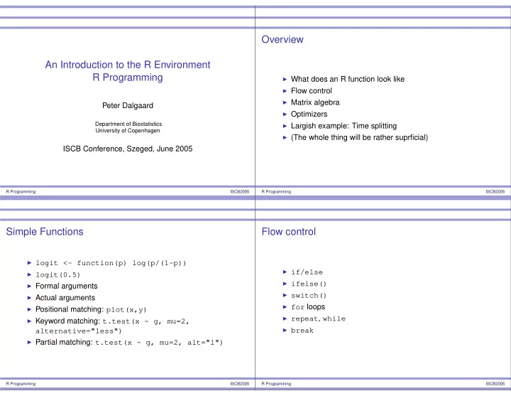
SLIDE 1 An Introduction to the R Environment R Programming
Peter Dalgaard
Department of Biostatistics University of Copenhagen
ISCB Conference, Szeged, June 2005
R Programming ISCB2005
Overview
◮ What does an R function look like ◮ Flow control ◮ Matrix algebra ◮ Optimizers ◮ Largish example: Time splitting ◮ (The whole thing will be rather suprficial)
R Programming ISCB2005
Simple Functions
◮ logit <- function(p) log(p/(1-p)) ◮ logit(0.5) ◮ Formal arguments ◮ Actual arguments ◮ Positional matching: plot(x,y) ◮ Keyword matching: t.test(x ~ g, mu=2,
alternative="less")
◮ Partial matching: t.test(x ~ g, mu=2, alt="l")
R Programming ISCB2005
Flow control
◮ if/else ◮ ifelse() ◮ switch() ◮ for loops ◮ repeat, while ◮ break
R Programming ISCB2005
SLIDE 2 Apply-functions/loop avoidance
◮ lapply – list-apply ◮ sapply – simplifying apply ◮ tapply – tabulating apply ◮ apply, sweep – along slices of tables ◮ replicate – repeat expression
R Programming ISCB2005
Matrix algebra
◮ R contains a pretty full set of primitives for matrix calculus ◮ A %*% B for matrix multiplication ◮ solve(A, b) for solving linear equations. (solve(A) for
matrix inverse)
◮ Various special products and decompositions
R Programming ISCB2005
Example of Matrix Code
Code to calculate the Greenhouse-Geisser epsilon:
Psi <- T %*% Sigma %*% t(T) B <- T %*% object$SSD %*% t(T) pp <- nrow(T) U <- solve(Psi,B) lambda <- Re(eigen(U)$values) GG.eps <- sum(lambda)^2/sum(lambda^2)/pp
R Programming ISCB2005
Optimization Tools
◮ 1-dimensional: optimize ◮ nlm, Newton-style optimizer ◮ optim, wrapper for several advanced optimizers
R Programming ISCB2005
SLIDE 3 Demo 1
mll <- function(theta) -dbinom(4, 10, theta, log=TRUE) plot(mll)
nlm(mll, .5)
- ptim(.5, mll, method="BFGS")
R Programming ISCB2005
Example: Time Splitting
◮ Split survival data into bands according to some time scale ◮ Used in survival analysis and epidemiology ◮ Vector of (delayed-entry) survival times ◮ Vector of break points ◮ (Possibly) individual origin of time scale for splitting
R Programming ISCB2005
“The SAS Way”
(pseudocode)
loop over individuals (implicit) loop over intervals { if overlap with survival time { trim survival time to interval
} }
R Programming ISCB2005
The R Way
Might mimic the SAS strategy, but it is inefficient in R. Here’s another idea:
loop over intervals { select subjects that overlap with interval trim times to interval keep resulting vector } stick all vectors together
That way, we can utilize vectorization of the selection and trimming tasks.
R Programming ISCB2005
SLIDE 4 Trimming to a Single Interval
◮ Survival: time1, time2, event ◮ Interval: left, right ◮ Turns out to be easier to "shoot first and ask questions
later" about the overlap:
en <- pmax(time1, left) ex <- pmin(time2, right) ev <- event & (time2 <= right) valid <- (en < ex) Surv(en[valid], ex[valid], ev[valid])
Notice that left and right can be vectors and incorporate a subject-specific origin.
R Programming ISCB2005
Trimming as Function
trimToI <- function(I) { left <- I[1] + origin ; right <- I[2] + origin en <- pmax(time1, left) ex <- pmin(time2, right) ev <- event & (time2 <= right) valid <- (en < ex) data.frame(S=Surv(en[valid], ex[valid], ev[valid]), subj=subj[valid]) }
This is designed to be defined inside the actual timesplit
- function. Notice that some variables are left to be bound via
lexical scope.
R Programming ISCB2005
Processing All Time Bands
We want to use some sort of apply-function and collect results as list of data frames. Here’s a nice way:
nbrk <- length(brks) Imat <- cbind(brks[-nbrk], brks[-1]) l <- apply(Imat, 1, trimToI)
and then just stick things together with
result <- do.call("rbind", l)
as it turns out, you need to do a little bit more because the rbind turns the Surv objects into matrices.
R Programming ISCB2005
Describing the Timebands
The output from our timesplitting function should contain a variable describing to which time band each piece belongs (this is not obvious if the origin differs between individuals) Getting the result as a factor with the proper level set is a little
lbl <- apply(Imat, 1, function(I) paste("(",I[1],",", I[2],"]", sep="")) f <- factor(lbl, levels=lbl) # avoid level sorting rep(f, lapply(l, nrow))
Next slide gives the final function.
R Programming ISCB2005
SLIDE 5
timesplit <- function(S, brks, origin=0, subj=1:nrow(S)) { time1 <- S[,1] ; time2 <- S[,2] ; event <- S[,3] trimToI <- function(I) { left <- I[1] + origin ; right <- I[2] + origin en <- pmax(time1, left) ex <- pmin(time2, right) ev <- event & (time2 <= right) valid <- (en < ex) data.frame(S=Surv(en[valid], ex[valid], ev[valid]), subj=subj[valid]) } nbrk <- length(brks) Imat <- cbind(brks[-nbrk], brks[-1]) l <- apply(Imat, 1, trimToI) result <- do.call("rbind", l) attr(result$S, "type") <- "counting" class(result$S) <- "Surv" lbl <- apply(Imat, 1, function(I) paste("(",I[1],",", I[2],"]", sep="")) f <- factor(lbl, levels=lbl) # avoid level sorting issues cbind(result, band=rep(f, lapply(l, nrow))) }