Overload handling methods Local Local Global Global Are - - PDF document

SLIDE 1

1

Overload handling methods

Reactive Let the overload to

• ccur and react to

contain its effects. Reactive Let the overload to

• ccur and react to

contain its effects. Proactive Prevent the overload to

• ccur by reducing the

computational request. Proactive Prevent the overload to

• ccur by reducing the

computational request. Local Are implemented as an adaptive behavior of application tasks. Local Are implemented as an adaptive behavior of application tasks. Global Are part of the system and can act on the task set and on the kernel. Global Are part of the system and can act on the task set and on the kernel.

Local Policies

ei Ri dmissi …

i

mechanisms probes

Real-Time System state variables Controlled Plant

sensors sensors

They are implemented inside specific application tasks as an adaptive behavior to reduce their computational demand:

adaptive task

Global Policies

Load estimator Load estimator Policy Policy

mechanisms probes

(t)

task set parameters

Real-Time System They are implemented as a component (Overload Manager) that can operate both on the kernel and on the entire task set: Task Set Task Set

actual exec. times ei response times Ri deadline misses

Overload Manager

Reactive methods

They let the overload to occur, detect it and react with a proper action aimed at containing its effects. They let the overload to occur, detect it and react with a proper action aimed at containing its effects. They must handle three phases:

• 1. Overload detection: this is done by proper kernel probes and

timers for catching deadline misses, execution overruns, etc.

• 2. Exception notification: this is done by generating an interrupt for

the kernel and a message for the user.

• 3. Exception handling: depending on the criticality of the exception,

possible actions are:

• system reset
• abortion of the running task
• rejection of least important tasks
• performance degradation
• no action: just notification

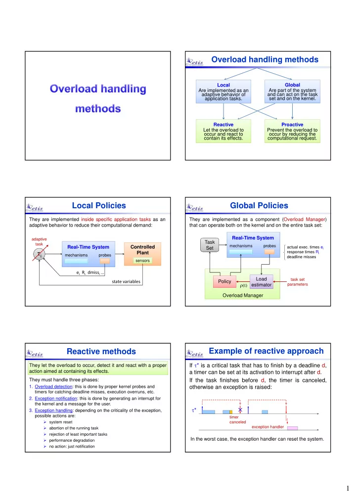
Example of reactive approach

If * is a critical task that has to finish by a deadline d, a timer can be set at its activation to interrupt after d. If the task finishes before d, the timer is canceled,

• therwise an exception is raised:

*

exception handler timer canceled

In the worst case, the exception handler can reset the system.

SLIDE 2

2

Proactive methods

They prevent the overload to occur by proper admission tests and by reducing the computational demand of the application. They prevent the overload to occur by proper admission tests and by reducing the computational demand of the application. The computational demand can be reduced by:

• rejecting tasks
• reducing computation
• reducing priority (under fixed priority systems)
• postponing the deadline (under deadline-based systems)
• skipping specific jobs
• reducing the activation rate of periodic tasks

Depending on the type of performed action, the following proactive approaches can be distinguished:

• Admission control methods

The load is reduced by rejecting one or more tasks.

• Performance degradation methods

The load is reduced by degrading the system performance acting on the task set parameters (computation times, periods, or skipping specific jobs).

• Resource Reservation methods

The load of each task is contained by a proper isolation mechanism that delays only those tasks experiencing the

• verrun, without affecting the other tasks.

Existing proactive approaches Simple admission control

Real-Time System Real-Time System The load is estimated at every task activation based on worst- case task set parameters: if   1, the task is accepted,

• therwise it is rejected:

Task Set Task Set  > 1

Load estimator Load estimator

NO YES

i

reject i

Pros: Simplicity (like the telephone system). Accepted tasks are guaranteed to receive full service. Pros: Simplicity (like the telephone system). Accepted tasks are guaranteed to receive full service. Cons: Load estimation is pessimistic (using WCETs and MITs) so tasks could be unnecessarily rejected. Task importance is not taken into account. Cons: Load estimation is pessimistic (using WCETs and MITs) so tasks could be unnecessarily rejected. Task importance is not taken into account.

Admission by feedback

Real-Time System Real-Time System The load is estimated at every task activation based on actual execution behavior detected by kernel probes [Stankovic, '99]: Task Set Task Set  > 1

Load estimator Load estimator

NO YES

i

reject i

Pros: It increases system efficiency, accepting more tasks. Pros: It increases system efficiency, accepting more tasks. Cons: Tasks can experience deadline misses (not good for safety-critical systems). Task importance is not taken into account. Cons: Tasks can experience deadline misses (not good for safety-critical systems). Task importance is not taken into account.

probes

ei Ri dmissi …

Taking value into account

How to take task importance into account?

• Under RM and EDF, the value of a task is implicitly

encoded in its period or its deadline.

• However, in a chemical plant controller, a task reading

the steam temperature every 10 seconds is more important than a graphic task that updates the clock icon every second.

Then, should we schedule tasks based on their importance value? Then, should we schedule tasks based on their importance value?

Highest Value First

A possible scheduling algorithm could schedule tasks based on their importance value (Highest Value First):

i

CPU READY queue READY queue

• rdered by value
• This policy guarantees that high importance tasks are

always executed.

• However, system efficiency could be quite low.

SLIDE 3

3 Considering only value is not good

Guaranteeing the execution of high importance tasks is a good thing in a RT system, but considering

• nly

importance is not efficient:

high value low value Scheduler: Highest Value First high value low value Scheduler: Earliest Deadline First

Only deadline is not good either

In overload conditions, EDF is not optimal:

high value low value A better schedule achieving more value Schedule produced by EDF high value low value

How to use value?

• If   1, EDF is optimal (value is not needed).
• If  > 1, all tasks cannot finish within their deadline.

 To avoid domino effects, the load has to be reduced, hence some task has to be rejected.  We would like to reject the least important tasks.

To manage overload conditions, the system must be able to handle tasks with both timing constraints and importance value. To manage overload conditions, the system must be able to handle tasks with both timing constraints and importance value.

Robust EDF scheduling

Recovery Policy Recovery Policy

probes

The load is estimated at every task activation: if   1, the task is accepted, otherwise the overload manager is invoked. Task Set Task Set  > 1

Load estimator Load estimator

NO YES

i

Reject Policy Reject Policy

Real-Time System

READY queue READY queue

Separated policies

• Tasks are scheduled by deadline and rejected by value.
• Under early completions, rejected tasks can be recovered.

2 4 6 8 10 12 14

1 2 5 3 4

16 18

Vi 7 10 5 2 3

20

Example: task rejection

At time t = 4, the arrival of 1 generates an overload. Which task should be rejected?

2 4 6 8 10 12 14

1 2 5 3 4

16 18

Vi 7 10 5 2 3

20

Example: task rejection

3 is the least value task that, if rejected,

can resolve the overload.

3 is the least value task that, if rejected,

can resolve the overload.

SLIDE 4

4

2 4 6 8 10 12 14

1 2 5 3 4

16 18

Vi 7 10 5 2 3

20

Example: task rejection

Lmax = 3 d* = 13

 = {1, 2, 3}  rej = 3

the least value task in Rejection policy: if d* is the first deadline miss after t, reject

 = {i | (di  d*) AND (ci(t)  Lmax)}

Example: task recovery

2 4 6 8 10 12 14

1 2 5 3 4

16 18

at time t = 8, 3 units are saved  3 can be recovered

20

1 2

Vi 7 10 5 2 3

Performance evaluation

Every time a task is completed, the system accumulates a score, which depends on

• the task value
• the time at which the task is finished.

How can we evaluate the performance of different scheduling algorithm in overload conditions? How can we evaluate the performance of different scheduling algorithm in overload conditions?

vi = Vi arbitrary constant vi = Ci computation time vi = Vi / Ci value density

A value vi can be assigned according to different criteria:

Value as a function of time

In a real-time system, the value of a task depends

• n its completion time and criticality:

vi (fi) fi

soft

vi (fi) fi

firm di di ri ri

vi (fi) fi

hard di ri

• 

vi (fi) fi

target sensitive di ri

Performance evaluation

The performance of a scheduling algorithm A on a task set T can be evaluated by computing the Cumulative Value:

) ( ) (

1





 

n i i i A

f v T

• Note that, in overload conditions:





   

n i i A

V

1 max

) ( ) ( T T

Optimality under overloads

) ( max ) (

*

T T

A A 

 

Hence, the performance of an algorithm can be evaluated with respect to *. In overload conditions, there are no optimal

• n-line

algorithms able to guarantee a cumulative value equal to *. In overload conditions, there are no optimal

• n-line

algorithms able to guarantee a cumulative value equal to *. The maximum value that can be accumulated is:

SLIDE 5

5

Proof (assume: Vi = Ci)

A can only be maximized by knowing the future.

2 6 8 4 10 12 14 16

10 6 6

1 2 3

A = 10

If at time t = 0, r3 is not known, we cannot select the task that maximizes the cumulative value.

2 6 8 4 10 12 14 16

10 6 6

1 2 3

A = 12

2 6 8 4 10 12 14 16

10 6 6

1 2 3

A = 16

Proof (assume: Vi = Ci) Competitive Factor

 Let * be the maximum cumulative value achievable by an optimal clairvoyant algorithm.  An algorithm A has a competitive factor A, if it is guaranteed that, for any task set, it achieves: A  A *

) ( ) ( min

* T

T

T

  

A A



 Hence, A  [0,1] and can be computed as:

Competitive factor of EDF

 It is easy to show that EDF = 0: 1 2

V1 = K V2 = K

In such a situation, EDF = V2 and * = V1, hence EDF / * = V2 / V1  0 for V1 >> V2

A theoretical upper bound

[ Baruah et al., 91 ] If   2 and i Vi = Ci, then no on-line algorithm can have a competitive factor greater than 0.25. If   2 and i Vi = Ci, then no on-line algorithm can have a competitive factor greater than 0.25. This result can be formally proved by using an adversary argument, assuming that an

• nline

algorithm competes with a clairvoyant scheduler.

vi (fi) fi

firm di ri

Ci This results assumes a firm task model:

The adversary generates 2 types of tasks: – Major tasks: Ci = Di, ri+1 = di   – Associated tasks: Ci = , ri+1 = di

• • •
• • •

major tasks associated tasks

Ci Ci+1 (note:  = 2)

Task generation strategy

SLIDE 6

6

• If the player decides to abort a major task in favor of an

associated task, the adversary interrupts the sequence of associated tasks.

major tasks associated tasks

Ci on  

Task generation strategy

• If the player decides to complete i, the game terminates

with the generation of i+1.

• • •
• • •

Ci Ci+1 on  Ci



 

 

1 * i j j

C

Task generation strategy

major tasks associated tasks

• Since the overload must have a finite duration, the game

terminates with m (with m finite). NOTE: The player can complete at most one task:  if it schedules an associated task, it gets on =   if it schedules a major task, it gets on = Ci NOTE: The player can complete at most one task:  if it schedules an associated task, it gets on =   if it schedules a major task, it gets on = Ci Viceversa, the adversary can accumulate:  either executing all associated tasks  or alternating major tasks with associated tasks. Viceversa, the adversary can accumulate:  either executing all associated tasks  or alternating major tasks with associated tasks.



 

 

1 * i j j

C

Task generation strategy Critical sequence

• Let

0, 1, 2, …, i, i+1, …, m

be the longest sequence of major tasks generated by the adversary.

• If the player schedules i, it gets:



 

   

1 * i j j i

• n

C e C





 



1

) (

i j j i

• n

C C i 

 To create problems to the player the next task must be generated so that:

on(i+1)  on(i);

 On the other hand, to convince the player to continue, it must be:

on(i+1)  on(i);

 To create problems to the player the next task must be generated so that:

on(i+1)  on(i);

 On the other hand, to convince the player to continue, it must be:

on(i+1)  on(i);

• Hence, the worst possible sequence for the player is

such that: on(i+1)  on(i).

• Let 1/k be such a value. Then, if C0  1, the worst-case

sequence must be such that:

k C C

i j j i

1

1





 

That is:



 

 

i j j i i

C kC C

1

1

0 

C

Critical sequence

• If the player decides to schedule m we have:





   

m j j m

• n

C C

*









m j j m

• n

C C m ) ( 

• Thus, if there exists an m such that

k m

• n

1 ) (  

we can claim that

i k i

• n

  1 ) ( 

which means that the competitive factor of a on-line algorithm cannot be grater than 1/k.

Competitive Factor

SLIDE 7

7

 Note that on(m) is equal to:

1 1 1 1 1

) (

        

     

   

m m m j j m m j j m m m j j m m j j m

kC C C kC C C C C C C C

 Hence, condition on(m)  1/k is equivalent to:

k kC C

m m

1

1







Cm  Cm-1

Competitive Factor

It is possible to prove that the sequence:



 

 

i j j i i

C kC C

1

1

0 

C

diverges for k  4, that is  m such that Cm  Cm-1 Instead, for k < 4,  m such that Cm  Cm-1 hence, the player can never get on > 1/4.

Competitive Factor

In general, the upper bound of the competitive factor is a function of the load and varies as follows:

1 2



0.25 0.5 0.75 1

on

Competitive Factor

?

[Baruah et al., 91]: if 1 < ρ ≤ 2, then on  p, where p satisfies 4[1 − (ρ − 1)p]3 = 27p2

Performance degradation

The load can be decreased not only by rejecting tasks, but also by reducing their performance

• requirements. This can be done by:
• Degrading functionality (reducing task code)
• Skipping specific jobs
• Increasing periods

Functional degradation

In many applications, computation can be performed at different level of precision: the higher the precision, the longer the computation. Examples are:

• Binary search algorithms
• Image processing and computer graphics
• Neural learning
• Any time control

Imprecise computation

In this model, each task i (Ci, Di, wi) is divided in two parts:

 a mandatory part: m

i (Mi, Di)

 an optional part: o

i (Oi, Di)

Mi Oi Di

 Ci = Mi + Oi  wi = importance weight

SLIDE 8

8

In this model, a schedule is said to be:

 feasible, if all mandatory parts complete within Di  precise, if also the optional parts are completed.

Mi Oi i error: i = Oi  i average error:





  

n i i i a

w

1

GOAL: minimize the average error

Imprecise computation

i

Multiple versions

If a task does not comply with the imprecise computational model, another option is to implement a function in multiple versions (operational modes):

Mode 1 Mode 2 Mode 3

Ci

1

Ci

2

Ci

3

decreasing performance PID Sliding mode Model-predictive

Sensitivity Analysis

Given an unschedulable task set, the problem is:

WCET2 WCET1

T2 T1

Which Ci’s should be changed and how much? Which Ci’s should be changed and how much?

d

U T C T C  

2 2 1 1

         

2 2 1 1

T C U T C

d

If we require the total utilization to be equal to a desired value Ud we have:

UdT2 UdT1 Feasible region EDF bound C1 C2 Still we have to select one among the infinite number of solutions

Functional degradation

This method can be implemented both:

• globally: if the mode is selected by the overload manager
• locally:

if the mode is selected by the task itself

while (1) { // periodic loop i = 0; // modes m  [1,M] do { // select the best feasible mode i = i + 1; rho = estimate_load(mode[i]); } while ((rho > 1) && (i < M)); if (rho > 1) exception(UNFEASIBLE); execute(mode[i]); wait_for_next_period(); }

Example of local overload management

Global methods

Global methods can find the optimal solution taking task constraints into account:

WCET2 WCET1

T2 T1 UdT2 UdT1 Feasible region Input: C = vector of computation times

f

= vector of activation rates

dc = direction versor for downgrading C U

= actual task set utilization (U > 1)

Ud = final desired utilization (Ud  1)

C C2 C1 C’ dc Output:  = amount of downgrading

Global methods

WCET2 WCET1

T2 T1 UdT2 UdT1 Feasible region 1. Given computation times C and rates f 2. Select a direction dc for downgrading C 3. Set a desired utilization Ud 4. Compute a feasible point C’ = C + dc such that C’  f = Ud C C2 C1 C’ dc

General approach:

Ud – Cf dcf  =

SLIDE 9

9

Local methods

Local methods cannot find the optimal solution and can downgrade more than needed.

T2 T1 UdT2 UdT1 Feasible region C1

WCET2 WCET1 case in which 1 reacts before 2 case in which 1 reacts before 2

Local methods cannot find the optimal solution and can downgrade more than needed.

T2 T1 C2

Local methods

WCET2 WCET1 case in which 1 and 2 react simultaneously case in which 1 and 2 react simultaneously

UdT2 UdT1 C1 Feasible region

Imprecise computation

WCET2 WCET1

T2 T1 UdT2 UdT1 C C2 M2 C1 M1

case in which the local method does not work case in which the local method does not work

The variability range is continuous but limited by the mandatory parts.

Multiple versions

WCET2 WCET1

T2 T1 UdT2 UdT1 C

case in which the local method does not work case in which the local method does not work

The variability range is larger, but discrete.

C2

1

C3

1

C1

1

C3

2

C2

2

C1

2

Performance Optimization

WCET2 WCET1 Global methods can optimize system performance, provided that a performance index  can be computed as a function of the design parameters:



Imprecise computation

WCET2 WCET1

T2 T1 UdT2 UdT1 C C2 M2 C1 M1

The variability range is continuous but limited by the mandatory parts.

• ptimal

point

SLIDE 10

10

Multiple versions

WCET2 WCET1

T2 T1 UdT2 UdT1 C

The variability range is larger, but discrete.

C2

1

C3

1

C1

1

C3

2

C2

2

C1

2

• ptimal

point

Multiple versions

WCET2 WCET1

T2 T1 UdT2 UdT1 C C2

1

C3

1

C1

1

C3

2

C2

2

C1

2

If optimizing in the continuous space, the optimal solution must be searched for all discrete points around it.

• ptimal

point

If we have n tasks there are 2n points to be checked. If we have n tasks there are 2n points to be checked.

Sensitivity Analysis

The presented analysis is valid under EDF for tasks with D = T.

• Under fixed priorities for tasks with arbitrary deadlines the

problem is more complex and has been addressed by:

Enrico Bini, Marco Di Natale, and Giorgio Buttazzo, "Sensitivity Analysis for Fixed-Priority Real-Time Systems", Real-Time Systems, Vol. 39, No. 1-3, pp. 5-30, August 2008.

• Under EDF for tasks with arbitrary deadlines the problem is

more complex and has been addressed by:

Enrico Bini and Giorgio Buttazzo, "The space of EDF deadlines: the exact region and a convex approximation", Real-Time Systems, Vol. 41, No. 1, pp. 27-51, January 2009.

Engine control tasks

Version 1: reducing the number of functions

Mode Speed range (rpm) Functions WCET 1 [500, 2000) f1() , f2(), f3() C1 2 [2000, 4000) f1(), f2() C2 3 [4000, 6000] f1() C3 f1,f2,f3 f1,f2 f1

2000 4000 6000

rpm C() C1 C2 C3

500

Engine control tasks

Version 1: reducing the number of functions

#define W1 2000 #define W2 4000 #define W3 6000 task engine_control { while (1) { w = current_enging_speed(); if (w  W3) f1(); if (w < W2) f2(); if (w < W1) f3(); } wait_for_next_period(); } #define W1 2000 #define W2 4000 #define W3 6000 task engine_control { while (1) { w = current_enging_speed(); if (w  W3) f1(); if (w < W2) f2(); if (w < W1) f3(); } wait_for_next_period(); }

f1,f2,f3 f1,f2 f1

2000 4000 6000

rpm C()

500

Engine control tasks

Version 2: M operating modes with hysteresis

Mode Speed range (rpm) Functions WCET 1 [500, 2500] f1() C1 2 [2000, 4500) f2() C2 3 [4000, 6000] f3() C3

2000 4000 6000

rpm C() C1 C2 C3

500 2500 4500

SLIDE 11

11

Engine control tasks

//Global variables mode[M] = {f1(), f2(), f3()}; wh[M] = {2500, 4500, 6000}; wl[M] = { 500, 2000, 4000}; m = 1; // modes m  [1,M] task engine_control { w = current_enging_speed(); while (w > wh[m]) m = m+1; while (w < wl[m]) m = m-1; execute(mode[m]); } //Global variables mode[M] = {f1(), f2(), f3()}; wh[M] = {2500, 4500, 6000}; wl[M] = { 500, 2000, 4000}; m = 1; // modes m  [1,M] task engine_control { w = current_enging_speed(); while (w > wh[m]) m = m+1; while (w < wl[m]) m = m-1; execute(mode[m]); }

f1 f2 f3

2000 4000 6000

rpm C()

500

Version 2: M operating modes with hysteresis

Job skipping

Periodic load can also be reduced by skipping some jobs, once in a while.

Many systems tolerate skips, if they do not occur too often:

• multimedia systems (video reproduction)
• inertial systems (robots)
• monitoring systems (sporadic data loss)

skip skip skip

Example

1 17 . 1 6 4 2 1    

p

U The system is

• verloaded,

but tasks can be schedulable if 1 skips one instance every 3:

1

skip skip skip

2

FIRM task model

• Every

job can either be executed within its deadline, or completely rejected (skip).

• A

percentage

• f

task instances must be guaranteed off line to finish in time.

• Each task i is described by (Ci, Ti, Di, Si):

Si specifies the minimum number of jobs between two consecutive skips (Si = 2, ..., ).

• Si = 2 means skipping at most one job every two jobs;
• Si =  means that no skips are allowed.
• Every instance can be red or blue:

– red instances must finish within their deadline – blue instances can be aborted

• If a blue instance is aborted, the next Si  1

instances must be red.

• If a blue instance is completed within its deadline,

the next instance is still blue.

• The first Si  1 instances of every task must be red.

FIRM task model

i

Ci = 1 Ti = 2 Di = 2 Si = 3

skip skip skip skip

i

skip skip skip

Example

SLIDE 12

12

 

Local adaptation

A local adaptation approach is also possible for a task to comply with the assigned reservation:

i

Reservation Ci Ti Si Local Policy Local Policy

probes

Real-Time System

Equivalent utilization factor

L L g U

n i i L p



 



1 *

) , ( max

i i i i i

C S T L T L L g           ) , (

Schedulability Analysis

Theorem: A set of firm periodic tasks is schedulable by EDF if

1

*  p

U

A sufficient condition

A necessary condition

Theorem: A set of firm periodic tasks is not schedulable if

1 ) 1 (

1

 



 n i i i i i

S T S C

NOTE: the sum represents the utilization of the computation that must take place.

Bandwidth saving

• In general, skipping jobs of periodic tasks causes

a bandwidth saving:

• Such a bandwidth can be used for
• improving aperiodic responsiveness (by increasing

their reserved bandwidth);

• accepting a larger number of periodic tasks.

* p p

U U U   

In this case: Up

* = 1

In fact, for L = Ti we have gi (0,L) = Ci = Ti Hence: 1 ) , (  

i i i

T T L L g

Ci = Ti Ti

i

skip skip

Not always skips save bandwidth

SLIDE 13

13

In fact: g(0, T1) = T1 and g(0, T2) = T2 However, notice that in this case we still have Up

* = 1

Hence: 1 ) , ( ) , (

2 2 1 1

  T T g T T g

C1 = T1 T1

1

C2 = T1 T2

2

Not always skips save bandwidth

Relaxing timing constraints

• The idea is to reduce the load by increasing task

periods.

• Each task must specify a period range [Tmin, Tmax]

compatible with its function.

• Periods

are increased during

• verloads,

and reduced when the overload is over. Many control applications require tasks running at variable rates, to cope with changing conditions. Many control applications require tasks running at variable rates, to cope with changing conditions.

75

Example

96 . 70 15 40 10 20 10    

p

U task Ci Tmin Tmax

1 2 3

10 10 15 20 40 70 25 50 80 The task set is feasible with EDF If 4 arrives (C4 = 5, T4 = 30) the system is not schedulable: 13 . 1 30 5 70 15 40 10 20 10     

p

U 99 . 30 5 80 15 50 10 23 10     

p

U But, there exists a feasible schedule within the specified ranges:

Lot of feasible solutions

In general, there can be a lot of feasible solutions with periods inside the specified range, the problems is: How do we select a solution among all feasible ones? How do we select a solution among all feasible ones?

T1 T2 C2 C1 T1-min T1-max T2-min T2-max Feasible region

Sensitivity Analysis

f2 f1

1/C2 1/C1

d

U f C f C  

2 2 1 1 1 2 2 1

C f C U f

d 



If we require the total utilization to be equal to a desired value Ud we have:

Ud/C2 Ud/C1 Feasible region EDF bound

We can follow the same approach used for reducing computation times, in the rate-space:

f

f2 f1

1/C2 1/C1 Ud/C2 Ud/C1 Feasible region 1. Given computation times C and rates f 2. Select a direction df for downgrading f 3. Set a desired utilization Ud 4. Compute a feasible point f’ = f + df such that C  f’ = Ud f f2 f1 f’ df

General approach:

Ud – Cf C df  =

Sensitivity Analysis

How do we choose the direction df?

SLIDE 14

14

Finding a solution

• One approach is to use optimization techniques to

maximize a performance index.

• Another

approach is to assign each task an additional parameter specifying its flexibility to be adapted.

f2 f1

• ptimal

point

• Tasks’ utilizations are treated as elastic springs and can be

changed by period variations.

• The flexibility of a task to a period variation is controlled by

an elastic coefficient Ei (the higher Ei the greater the elasticity).

• A periodic task i is characterized by: (Ci, Ti , Ti , Ei)

Ei ri Ti t

i

Ti Ti

Elastic task model

min max min max

Special cases

• A task with T min = T max is equivalent to a hard task.
• A task with Ei = 0 can intentionally change its

period but does not allow the system to do that. Definitions

min max i i i

T C U 

max min i i i

T C U 







n i i

U U

1 max max







n i i

U U

1 min min

Compression algorithm

1 2 3 4

1

Up

1

Up

1 2 3 4 During overloads, utilizations must be compressed to bring the load below one.

The spring analogy

xi0 x x xi F

An elastic task can be compared with a linear spring:

spring length  task utilization spring length  task utilization xi

min

xi0 Ui

max = Ci

Ti

min

Ui

min = Ci

Ti

max

ki 1 Ei

A periodic task set with maximum utilization Umax that must be reduced to a desired utilization Ud can be treated as a set of linear springs with initial length L0 that must be compressed to reach a desired length Ld.

The spring analogy

1 2 3 4

1

U Umax

1

U

1 2 3 4

Ud

SLIDE 15

15

Solving a linear spring system

x x1o x2o x3o L0 x x1 x2 x3 F Ld

F = k1(x1o - x1) F = k2(x2o - x2) F = k3(x3o - x3) x1 + x2 + x3 = Ld x1o + x2o + x3o = L0

Solution assuming xmin = 0

) ( ) ( ) 1 1 1 (

3 2 1 3 2 1 3 2 1

x x x x x x k k k F

• 

      

Summing the equations, we have:

) (

d

L L  

That is:

3 2 1

1 1 1 ) ( k k k L L F

d

   

Substituting F in the equations, we have: That is:

3 2 1 1 1 1

1 1 1 ) ( ) ( k k k L L x x k F

d

• 

    

3 2 1 1 1 1

1 1 1 1 ) ( k k k k L L x x

d

• 

   

Solution assuming xmin = 0

 



n i i

k K

1 //

1 1

i d io i

k K L L x x

//

) (   

And defining: Ei = 1/ki







n i i s

E E

1 s i d io i

E E L L x x ) (

0 

 

Solution assuming xmin = 0

s i d i i

E E U U U U ) (

max max

  

Solution assuming Tmax = 

s i d io i

E E L L x x ) (

0 

 

Interpreting the solution for a task set we have:

i i i

U C T 

Once the various Ui have been derived, task periods can be set as:

Solution with constraints

x L0 x F Ld x F Ld

If Tmax <  (i.e., xmin > 0), the solution becomes iterative, requiring at most n iterations:

SLIDE 16

16

v i f d v i i v i

E E U U U U U ) (

max max

      

After each step, the set  can be divided into two subsets:

• a set f of fixed springs that reached the minimum length;
• a set v of variable springs that can still be compressed.



 



v i

i v

U U

 max max



 



f i

i f

U U

 min



 



v i

i v

E E



If for some task Ui < Ui

min, then set Ui = Ui min, update

v and f and repeat the process.

Solution with constraints

• Feasibility condition

Observations (1)

• The

computational complexity

• f

the elastic compression algorithm is O(n2)

• Initialization values of the iterative process:

  v {}  f

max max

U Uv  

f

U

s v

E E 

Given a task set with Umax > Ud, a compressed solution always exists if and only if Umin  Ud. Given a task set with Umax > Ud, a compressed solution always exists if and only if Umin  Ud.

Observations (2)

• The compression algorithm can be used to adjust

periods every time a task is added to the system, or a task requests to adapt its period.

• The compression algorithm can also be used to

increase utilizations when the overload is over or when a task set underutilize the processor.

• Elastic compression can also be used to compute

how to reduce computation times (Ci = UiTi).

Experimental results

Overload handling due to a new task arrival:

time # of jobs 4 arrives at time ta ta 4 ends at time tb tb

3 2 1

Overload handling due to an increased rate:

time # of jobs 3 increases its rate at ta ta

Experimental results

3 decreases its rate at tb tb

1 2 3

Elastic Guarantee

Elastic Compression Elastic Compression

NO YES

*

exception

Umin  Ud

 =  U{*}  =  U{*}

Umax > Ud Real-Time System Real-Time System

Ud

Period Adaptation Period Adaptation

C

YES NO

T

end

 = \{*}  = \{*}