Outline Inventory (level) control structure Location of throughput - PowerPoint PPT Presentation

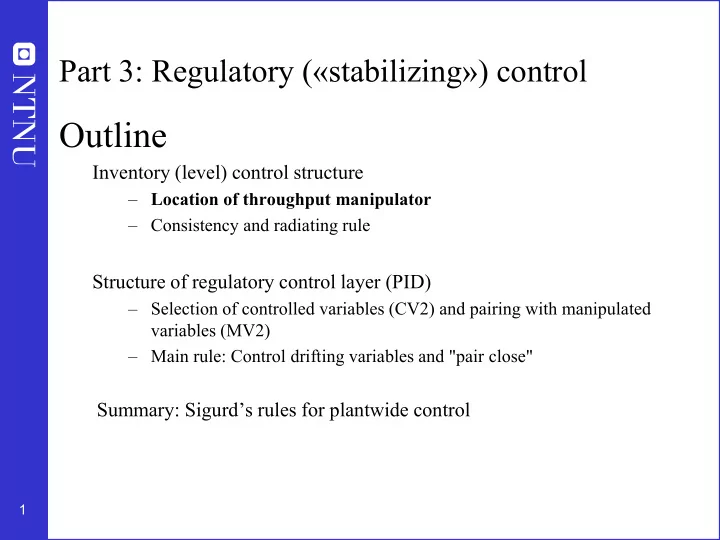
Part 3: Regulatory («stabilizing») control Outline Inventory (level) control structure – Location of throughput manipulator – Consistency and radiating rule Structure of regulatory control layer (PID) – Selection of controlled variables (CV2) and pairing with manipulated variables (MV2) – Main rule: Control drifting variables and "pair close" Summary: Sigurd ’ s rules for plantwide control 1

Procedure • Skogestad procedure for control structure design I Top Down • Step S1: Define operational objective (cost) and constraints • Step S2: Identify degrees of freedom and optimize operation for disturbances • Step S3: Implementation of optimal operation – What to control ? (primary CV ’ s) – Active constraints – Self-optimizing variables for unconstrained, c=Hy • Step S4: Where set the production rate? (Inventory control) II Bottom Up • Step S5: Regulatory control: What more to control (secondary CV ’ s) ? • Step S6: Supervisory control • Step S7: Real-time optimization 2

Step S4. Where set production rate? • Very important decision that determines the structure of the rest of the inventory control system! • May also have important economic implications • Link between Top-down (economics) and Bottom-up (stabilization) parts – Inventory control is the most important part of stabilizing control • “ Throughput manipulator ” (TPM) = MV for controlling throughput (production rate, network flow) • Where set the production rate = Where locate the TPM? – Traditionally: At the feed – For maximum production (with small backoff): At the bottleneck 3

TPM and link to inventory control • Liquid inventory: Level control (LC) – Sometimes pressure control (PC) • Gas inventory: Pressure control (PC) • Component inventory: Composition control (CC, XC, AC) 5

Production rate set at inlet : Inventory control in direction of flow* TPM * Required to get “ local-consistent ” inventory control 6

Production rate set at outlet: Inventory control opposite flow* TPM * Required to get “ local-consistent ” inventory control 7

Production rate set inside process* TPM * Required to get “ local-consistent ” inventory control 8

General: “ Need radiating inventory control around TPM ” (Georgakis) 9

Consistency of inventory control • Consistency (required property): An inventory control system is said to be consistent if the steady- state mass balances (total, components and phases) are satisfied for any part of the process, including the individual units and the overall plant. 10

QUIZ 1 CONSISTENT? Rule: Controlling pressure at inlet or outlet gives indirect flow control (because of pressure boundary condition) 13

LOCATION OF SENSORS • Location flow sensor (before or after valve or pump): Does not matter from consistency point of view – Locate to get best flow measurement • Before pump: Beware of cavitation • After pump: Beware of noisy measurement • Location of pressure sensor (before or after valve, pump or compressor): Important from consistency point of view 14

Example: Solid oxide fuel cell x CH4,s CC PC CH4 CH 4 + H 2 O = CO + 3H 2 CO + H 2 O = CO 2 + H 2 2H 2 + O 2- → 2H 2 O + 2e - H2O (in ratio with CH4 feed e - O 2- Solid oxide electrolyte TPM = current I [A] = disturbance to reduce C and CO formation) O 2 + 4e - → 2O 2- Air (excess O2) PC TC T s = 1070 K (active constraint) 23

Single-loop alternatives for bottleneck control Bottleneck. Traditional: Manual control of feed rate Want max flow here TPM Alt.1. Feedrate controls bottleneck flow (VPC: “ long loop ” with backoff … ): F max FC TPM Alt. 2: Feedrate controls lost task (another “ long loop ” ): MAX TPM Alt. 3: Reconfigure all upstream inventory loops: F max 28 TPM

Single-loop alternatives for bottleneck control Bottleneck. Traditional: Manual control of feed rate Want max flow here TPM Alt. 2: Feedrate controls level upstream bottleneck: MAX M3 TPM Comment on Alt. 2 where feed controls M3 . «Long loop», so slow. Can work if M3 is large, 29 Rule : Can keep TPM at feed if surge volume (M3) before bottleneck is large

Where should we place TPM? • TPM = MV used to control throughput • Traditionally: TPM = Main feed valve (or pump/compressor) – Gives inventory control “ in direction of flow ” Consider moving TPM if: 1. There is an important CV that could otherwise not be well controlled – Dynamic reasons – Special case: Max. production important: Locate TPM at process bottleneck* ! • TPM can then be used to achieve tight bottleneck control (= achieve max. production) • Economics: Max. production is very favorable in “ sellers marked ” 2. If placing it at the feed may yield infeasible operation ( “ overfeeding ” ) – If “ snowballing ” is a problem (accumulation in recycle loop), then consider placing TPM inside recycle loop BUT: Avoid a variable that may (optimally) saturate as TPM (unless it is at bottleneck) – Reason: To keep controlling CV=throughput, we would need to reconfigure (move TPM)** * Bottleneck: Last constraint to become active as we increase throughput -> TPM must be used for bottleneck control 30 **Sigurd ’ s general pairing rule (to reduce need for reassigning loops): “ Pair MV that may (optimally) saturate with CV that may be given up ”

Conclusion TPM (production rate manipulator) • Think carefully about where to place it! • Difficult to undo later 71

Session 5: Design of regulatory control layer 72

Outline • Skogestad procedure for control structure design I Top Down • Step S1: Define operational objective (cost) and constraints • Step S2: Identify degrees of freedom and optimize operation for disturbances • Step S3: Implementation of optimal operation – What to control ? (primary CV ’ s) (self-optimizing control) • Step S4: Where set the production rate? (Inventory control) II Bottom Up • Step S5: Regulatory control: What more to control (secondary CV ’ s) ? – Distillation example • Step S6: Supervisory control • Step S7: Real-time optimization 73

Regulatory layer Step 5. Regulatory control layer • Purpose : “ Stabilize ” the plant using a simple control configuration (usually: local SISO PID controllers + simple cascades) • Enable manual operation (by operators) • Main structural decisions: • What more should we control? (secondary cv ’ s, CV 2 , use of extra measurements) CV 1 • Pairing with manipulated variables (mv ’ s u 2 ) CV 2 = ? 75

Structure of regulatory control layer (PID) Main decisions: 1. Selection of controlled variables (CV2) 2. Pairing with manipulated variables (MV2) Main rules: 1. Control drifting variables CV2 ↕ 2. «Pair close" MV2 76

Regulatory layer Stabilizing control: Use inputs MV 2 =u 2 to control “ drifting ” variables CV 2 Primary CV CV 1 CV 2s u 2 K G CV 2 Secondary CV (control for dynamic reasons) Key decision : Choice of CV 2 (controlled variable) Also important : Choice of MV2=u 2 ( “ pairing ” ) Process control: Typical «drifting» variables (CV2) are • Liquid inventories (level) • Vapor inventories (pressure) • Some temperatures (reactor, distillation column profile) 77

Regulatory layer Degrees of freedom unchanged • No degrees of freedom lost as setpoints y 2s replace inputs u 2 as new degrees of freedom for control of y 1 Cascade control: CV 1 CV 2s u 2 K G CV 2 MV2=Original DOF CV2 s =New DOF 78

Regulatory layer Objectives regulatory control layer 1. Allow for manual operation 2. Simple decentralized (local) PID controllers that can be tuned on-line 3. Take care of “ fast ” control 4. Track setpoint changes from the layer above 5. Local disturbance rejection 6. Stabilization (mathematical sense) 7. Avoid “ drift ” (due to disturbances) so system stays in “ linear region ” – “ stabilization ” (practical sense) 8. Allow for “ slow ” control in layer above (supervisory control) 9. Make control problem easy as seen from layer above 10. Use “ easy ” and “ robust ” measurements (pressure, temperature) 11. Simple structure 12. Contribute to overall economic objective ( “ indirect ” control) 13. Should not need to be changed during operation 79

Regulatory layer Example: Exothermic reactor (unstable) Active constraints (economics): Product composition c + level (max) • u = cooling flow (q) • CV 1 = composition (c) • CV 2 = temperature (T) feed CV 1s CV 1 =c L s =max CC CV 2s LC CV 2 =T product TC u cooling 80

Regulatory layer “ Control CV2 that stabilizes the plant (stops drifting) ” In practice, control: 1. Levels (inventory liquid) 2. Pressures (inventory gas/vapor) (note: some pressures may be left floating) 3. Inventories of components that may accumulate/deplete inside plant • E.g., amine/water depletes in recycle loop in CO2 capture plant • E.g., butanol accumulates in methanol-water distillation column • E.g., inert N2 accumulates in ammonia reactor recycle 4. Reactor temperature 5. Distillation column profile (one temperature inside column) • Stripper/absorber profile does not generally need to be stabilized 85

Regulatory layer Main rule: “ Pair close ” The response (from input to output) should be fast, large and in one direction . Avoid dead time and inverse responses! 87