Outline Flexible, optimal matching for observational Optimal - - PowerPoint PPT Presentation

Flexible, optimal matching for observational studies

Ben Hansen University of Michigan 15 June 2006

Outline

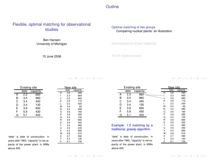
Optimal matching of two groups Comparing nuclear plants: an illustration Generalizations of pair matching The R implementation Existing site

date capacity A 2.3 660 B 3.0 660 C 3.4 420 D 3.4 130 E 3.9 650 F 5.9 430 G 5.1 420

“date” is date of construction, in years after 1965; “capacity” is net ca- pacity of the power plant, in MWe above 400.

New site

date capacity H 3.6 290 I 2.3 660 J 3.0 660 K 2.9 110 L 3.2 420 M 3.4 60 N 3.3 390 O 3.6 160 P 3.8 390 Q 3.4 130 R 3.9 650 S 3.9 450 T 3.4 380 U 4.5 440 V 4.2 690 W 3.8 510 X 4.7 390 Y 5.4 140 Z 6.1 730

Existing site

date capacity A 2.3 660 B 3.0 660 C 3.4 420 D 3.4 130 E 3.9 650 F 5.9 430 G 5.1 420

Example: 1:2 matching by a traditional, greedy algorithm.

“date” is date of construction, in years after 1965; “capacity” is net ca- pacity of the power plant, in MWe above 400.

New site

date capacity H 3.6 290 I 2.3 660 J 3.0 660 K 2.9 110 L 3.2 420 M 3.4 60 N 3.3 390 O 3.6 160 P 3.8 390 Q 3.4 130 R 3.9 650 S 3.9 450 T 3.4 380 U 4.5 440 V 4.2 690 W 3.8 510 X 4.7 390 Y 5.4 140 Z 6.1 730

Existing site

date capacity A 2.3 660 B 3.0 660 C 3.4 420 D 3.4 130 E 3.9 650 F 5.9 430 G 5.1 420

Example: 1:2 matching by a traditional, greedy algorithm.

“date” is date of construction, in years after 1965; “capacity” is net ca- pacity of the power plant, in MWe above 400.

New site

date capacity H 3.6 290 I 2.3 660 J 3.0 660 K 2.9 110 L 3.2 420 M 3.4 60 N 3.3 390 O 3.6 160 P 3.8 390 Q 3.4 130 R 3.9 650 S 3.9 450 T 3.4 380 U 4.5 440 V 4.2 690 W 3.8 510 X 4.7 390 Y 5.4 140 Z 6.1 730

Existing site

date capacity A 2.3 660 B 3.0 660 C 3.4 420 D 3.4 130 E 3.9 650 F 5.9 430 G 5.1 420

Example: 1:2 matching by a traditional, greedy algorithm.

“date” is date of construction, in years after 1965; “capacity” is net ca- pacity of the power plant, in MWe above 400.

New site

date capacity H 3.6 290 I 2.3 660 J 3.0 660 K 2.9 110 L 3.2 420 M 3.4 60 N 3.3 390 O 3.6 160 P 3.8 390 Q 3.4 130 R 3.9 650 S 3.9 450 T 3.4 380 U 4.5 440 V 4.2 690 W 3.8 510 X 4.7 390 Y 5.4 140 Z 6.1 730

Existing site

date capacity A 2.3 660 B 3.0 660 C 3.4 420 D 3.4 130 E 3.9 650 F 5.9 430 G 5.1 420

Example: 1:2 matching by a traditional, greedy algorithm.

“date” is date of construction, in years after 1965; “capacity” is net ca- pacity of the power plant, in MWe above 400.

New site

date capacity H 3.6 290 I 2.3 660 J 3.0 660 K 2.9 110 L 3.2 420 M 3.4 60 N 3.3 390 O 3.6 160 P 3.8 390 Q 3.4 130 R 3.9 650 S 3.9 450 T 3.4 380 U 4.5 440 V 4.2 690 W 3.8 510 X 4.7 390 Y 5.4 140 Z 6.1 730

Existing site

date capacity A 2.3 660 B 3.0 660 C 3.4 420 D 3.4 130 E 3.9 650 F 5.9 430 G 5.1 420

Example: 1:2 matching by a traditional, greedy algorithm.

“date” is date of construction, in years after 1965; “capacity” is net ca- pacity of the power plant, in MWe above 400.

New site

date capacity H 3.6 290 I 2.3 660 J 3.0 660 K 2.9 110 L 3.2 420 M 3.4 60 N 3.3 390 O 3.6 160 P 3.8 390 Q 3.4 130 R 3.9 650 S 3.9 450 T 3.4 380 U 4.5 440 V 4.2 690 W 3.8 510 X 4.7 390 Y 5.4 140 Z 6.1 730

Existing site

date capacity A 2.3 660 B 3.0 660 C 3.4 420 D 3.4 130 E 3.9 650 F 5.9 430 G 5.1 420

Example: 1:2 matching by a traditional, greedy algorithm.

“date” is date of construction, in years after 1965; “capacity” is net ca- pacity of the power plant, in MWe above 400.

New site

date capacity H 3.6 290 I 2.3 660 J 3.0 660 K 2.9 110 L 3.2 420 M 3.4 60 N 3.3 390 O 3.6 160 P 3.8 390 Q 3.4 130 R 3.9 650 S 3.9 450 T 3.4 380 U 4.5 440 V 4.2 690 W 3.8 510 X 4.7 390 Y 5.4 140 Z 6.1 730

Existing site

date capacity A 2.3 660 B 3.0 660 C 3.4 420 D 3.4 130 E 3.9 650 F 5.9 430 G 5.1 420

Example: 1:2 matching by a traditional, greedy algorithm.

“date” is date of construction, in years after 1965; “capacity” is net ca- pacity of the power plant, in MWe above 400.

New site

date capacity H 3.6 290 I 2.3 660 J 3.0 660 K 2.9 110 L 3.2 420 M 3.4 60 N 3.3 390 O 3.6 160 P 3.8 390 Q 3.4 130 R 3.9 650 S 3.9 450 T 3.4 380 U 4.5 440 V 4.2 690 W 3.8 510 X 4.7 390 Y 5.4 140 Z 6.1 730

New and refurbished nuclear plants: discrepancies in capacity and year of construction

Exist- New sites ing H I J K L M N O P Q R S T U V W X Y Z A 28 3 22 14 30 17 28 26 28 20 22 23 26 21 18 34 40 28 B 24 3 0 22 10 27 14 26 24 24 16 19 20 23 18 16 31 37 25 C 10 18 14 18 4 12 6 11 9 10 14 12 6 14 22 10 16 22 28 D 7 28 24 8 14 2 10 6 12 0 24 22 4 24 32 20 18 16 38 E 17 20 16 32 18 26 20 18 12 24 2 20 6 8 4 14 20 14 F 20 31 28 35 20 29 22 20 14 26 12 9 22 5 15 12 9 11 12 G 14 32 29 30 18 24 17 16 10 22 12 10 17 6 16 14 4 8 17

Existing site

date capacity A 2.3 660 B 3.0 660 C 3.4 420 D 3.4 130 E 3.9 650 F 5.9 430 G 5.1 420

Optimal vs. Greedy matching

By evaluating potential matches all together rather than sequentially, op- timal matching (blue lines) reduces the sum of distances from 82 to 63.

New site

date capacity H 3.6 290 I 2.3 660 J 3.0 660 K 2.9 110 L 3.2 420 M 3.4 60 N 3.3 390 O 3.6 160 P 3.8 390 Q 3.4 130 R 3.9 650 S 3.9 450 T 3.4 380 U 4.5 440 V 4.2 690 W 3.8 510 X 4.7 390 Y 5.4 140 Z 6.1 730

Introducing restrictions on who can be matched to whom: calipers

In the nuclear plants example, suppose we choose to insist upon a caliper of three years in the date of construction. This would forbid five potential matches, indicated below in red.

Exist- New sites ing H I J K L M N O P Q R S T U V W X Y Z A 28 3 22 14 30 17 28 26 28 20 22 23 26 21 18 34 40 28 B 24 3 0 22 10 27 14 26 24 24 16 19 20 23 18 16 31 37 25 C 10 18 14 18 4 12 6 11 9 10 14 12 6 14 22 10 16 22 28 D 7 28 24 8 14 2 10 6 12 0 24 22 4 24 32 20 18 16 38 E 17 20 16 32 18 26 20 18 12 24 2 20 6 8 4 14 20 14 F 20 31 28 35 20 29 22 20 14 26 12 9 22 5 15 12 9 11 12 G 14 32 29 30 18 24 17 16 10 22 12 10 17 6 16 14 4 8 17

Introducing restrictions on who can be matched to whom: calipers

With optmatch, matches are forbidden by placing ∞’s in the distance matrix.

Exist- New sites ing H I J K L M N O P Q R S T U V W X Y Z A 28 3 22 14 30 17 28 26 28 20 22 23 26 21 18 34 Inf Inf B 24 3 0 22 10 27 14 26 24 24 16 19 20 23 18 16 31 37 Inf C 10 18 14 18 4 12 6 11 9 10 14 12 6 14 22 10 16 22 28 D 7 28 24 8 14 2 10 6 12 0 24 22 4 24 32 20 18 16 38 E 17 20 16 32 18 26 20 18 12 24 2 20 6 8 4 14 20 14 F 20 Inf 28 Inf 20 29 22 20 14 26 12 9 22 5 15 12 9 11 12 G 14 32 29 30 18 24 17 16 10 22 12 10 17 6 16 14 4 8 17

Outline

Optimal matching of two groups Comparing nuclear plants: an illustration Generalizations of pair matching The R implementation

Example # 2: Gender equity study for research scientists1

Women and men scientists are to be matched on grant funding. Women Men Subject log10(Grant) Subject log10(Grant) A 5.7 V 5.5 B 4.0 W 5.3 C 3.4 X 4.9 D 3.1 Y 4.9 Z 3.9

1Discussed in Hansen and Klopfer (2005), Hansen (2004)

Full Matching2 the Gender Equity Sample

Women Men Subject log10(Grant) Subject log10(Grant) A 5.7 V 5.5 B 4.0 W 5.3 C 3.4 X 4.9 D 3.1 Y 4.9 Z 3.9

◮ Similar to matching with replacement, but creates disjoint

matched sets — better for tests & CIs.

◮ In contrast to pair matching, it finds matches for everyone

with a suitable counterpart.

◮ In contrast to multiple controls matching, it doesn’t force

poor matches.

◮ In optmatch, can be combined with structural restrictions.

2(Rosenbaum, 1991; Hansen and Klopfer, 2005)

Full Matching2 the Gender Equity Sample

Women Men Subject log10(Grant) Subject log10(Grant) A 5.7 V 5.5 B 4.0 W 5.3 C 3.4 X 4.9 D 3.1 Y 4.9 Z 3.9

◮ Similar to matching with replacement, but creates disjoint

matched sets — better for tests & CIs.

◮ In contrast to pair matching, it finds matches for everyone

with a suitable counterpart.

◮ In contrast to multiple controls matching, it doesn’t force

poor matches.

◮ In optmatch, can be combined with structural restrictions.

2(Rosenbaum, 1991; Hansen and Klopfer, 2005)

Full Matching2 the Gender Equity Sample

Women Men Subject log10(Grant) Subject log10(Grant) A 5.7 V 5.5 B 4.0 W 5.3 C 3.4 X 4.9 D 3.1 Y 4.9 Z 3.9

◮ Similar to matching with replacement, but creates disjoint

matched sets — better for tests & CIs.

◮ In contrast to pair matching, it finds matches for everyone

with a suitable counterpart.

◮ In contrast to multiple controls matching, it doesn’t force

poor matches.

◮ In optmatch, can be combined with structural restrictions.

2(Rosenbaum, 1991; Hansen and Klopfer, 2005)

Full Matching2 the Gender Equity Sample

Women Men Subject log10(Grant) Subject log10(Grant) A 5.7 V 5.5 B 4.0 W 5.3 C 3.4 X 4.9 D 3.1 Y 4.9 Z 3.9

◮ Similar to matching with replacement, but creates disjoint

matched sets — better for tests & CIs.

◮ In contrast to pair matching, it finds matches for everyone

with a suitable counterpart.

◮ In contrast to multiple controls matching, it doesn’t force

poor matches.

◮ In optmatch, can be combined with structural restrictions.

2(Rosenbaum, 1991; Hansen and Klopfer, 2005)

Outline

Optimal matching of two groups Comparing nuclear plants: an illustration Generalizations of pair matching The R implementation

Under the hood

Full matching via network flows3

T C

+U . . . −|C| . . . +U

|C| − nU

Sink Overflow

[0,1] [ , 1 ] [0,1] [0,1] [0, U − 1] [ , ˜ U − 1 ]

3(Hansen and Klopfer, 2005, Fig. 2). Time complexity of the algorithm is

O(n3 log(n max(dist))).

Arguments to fullmatch()

distance The argument demanding most attention from the user, b/c it defines “good” matches and because very large distance matrices can tax R’s memory

• limits. A new helper function, makedist(), eases

both of these efforts. min.controls, max.controls In propensity matching, can be important for efficiency — see Hansen (2004), Augursky and Kluve (2004).

• mit.fraction for use in matched sampling (as opposed to

matching all or most of a sample). Not needed for getting rid of subjects without suitable potential

• matches. If you’re not specifically out to reduce the

size of the control group, can be ignored.

Arguments to fullmatch()

distance The argument demanding most attention from the user, b/c it defines “good” matches and because very large distance matrices can tax R’s memory

• limits. A new helper function, makedist(), eases

both of these efforts. min.controls, max.controls In propensity matching, can be important for efficiency — see Hansen (2004), Augursky and Kluve (2004).

• mit.fraction for use in matched sampling (as opposed to

matching all or most of a sample). Not needed for getting rid of subjects without suitable potential

• matches. If you’re not specifically out to reduce the

size of the control group, can be ignored.

Arguments to fullmatch()

distance The argument demanding most attention from the user, b/c it defines “good” matches and because very large distance matrices can tax R’s memory

• limits. A new helper function, makedist(), eases

both of these efforts. min.controls, max.controls In propensity matching, can be important for efficiency — see Hansen (2004), Augursky and Kluve (2004).

• mit.fraction for use in matched sampling (as opposed to

matching all or most of a sample). Not needed for getting rid of subjects without suitable potential

• matches. If you’re not specifically out to reduce the

size of the control group, can be ignored.

Summary

◮ With optmatch, R offers the most comprehensive optimal

matching implementation for statistics.

◮ fullmatch() solves optimally such traditional problems

as matched sampling, pair matching, and matching with k controls.

◮ fullmatch() can also solve matching problems flexibly,

and far more effectively, by way of full matching, with or without structural restrictions (Hansen and Klopfer, 2005; Hansen, 2004).

◮ The effort required to code optimal and full matching

algorithms seems to have dissuaded their widespread use. Now that I’ve made that effort, perhaps this situation can change! :)

Summary

◮ With optmatch, R offers the most comprehensive optimal

matching implementation for statistics.

◮ fullmatch() solves optimally such traditional problems

as matched sampling, pair matching, and matching with k controls.

◮ fullmatch() can also solve matching problems flexibly,

and far more effectively, by way of full matching, with or without structural restrictions (Hansen and Klopfer, 2005; Hansen, 2004).

◮ The effort required to code optimal and full matching

algorithms seems to have dissuaded their widespread use. Now that I’ve made that effort, perhaps this situation can change! :)

Summary

◮ With optmatch, R offers the most comprehensive optimal

matching implementation for statistics.

◮ fullmatch() solves optimally such traditional problems

as matched sampling, pair matching, and matching with k controls.

◮ fullmatch() can also solve matching problems flexibly,

and far more effectively, by way of full matching, with or without structural restrictions (Hansen and Klopfer, 2005; Hansen, 2004).

◮ The effort required to code optimal and full matching

algorithms seems to have dissuaded their widespread use. Now that I’ve made that effort, perhaps this situation can change! :)

Summary

◮ With optmatch, R offers the most comprehensive optimal

matching implementation for statistics.

◮ fullmatch() solves optimally such traditional problems

as matched sampling, pair matching, and matching with k controls.

◮ fullmatch() can also solve matching problems flexibly,

and far more effectively, by way of full matching, with or without structural restrictions (Hansen and Klopfer, 2005; Hansen, 2004).

◮ The effort required to code optimal and full matching

algorithms seems to have dissuaded their widespread use. Now that I’ve made that effort, perhaps this situation can change! :)

Example with propensity scores and stratification prior to matching

>nuclear$pscore <- glm(pr~.-cost, + family=binomial(),data=nuclear)$linear.predictors > pscorediffs <- function(trtvar,data) { + pscr <- data[names(trtvar), ’pscore’] + abs(outer(pscr[trtvar],pscr[!trtvar], ’-’)) + } > psd2 <- makedist(pr~pt, nuclear, pscorediffs) > fullmatch(psd2) > fullmatch(psd2, min.controls=1, max.controls=3) > fullmatch(psd2, min=1, max=c(’0’=3, ’1’=2)) Jake Bowers’ and my RItools package provides

• diagnostics. . .

Example with propensity scores and stratification prior to matching

>nuclear$pscore <- glm(pr~.-cost, + family=binomial(),data=nuclear)$linear.predictors > pscorediffs <- function(trtvar,data) { + pscr <- data[names(trtvar), ’pscore’] + abs(outer(pscr[trtvar],pscr[!trtvar], ’-’)) + } > psd2 <- makedist(pr~pt, nuclear, pscorediffs) > fullmatch(psd2) > fullmatch(psd2, min.controls=1, max.controls=3) > fullmatch(psd2, min=1, max=c(’0’=3, ’1’=2)) Jake Bowers’ and my RItools package provides

• diagnostics. . .

Example with propensity scores and stratification prior to matching

>nuclear$pscore <- glm(pr~.-cost, + family=binomial(),data=nuclear)$linear.predictors > pscorediffs <- function(trtvar,data) { + pscr <- data[names(trtvar), ’pscore’] + abs(outer(pscr[trtvar],pscr[!trtvar], ’-’)) + } > psd2 <- makedist(pr~pt, nuclear, pscorediffs) > fullmatch(psd2) > fullmatch(psd2, min.controls=1, max.controls=3) > fullmatch(psd2, min=1, max=c(’0’=3, ’1’=2)) Jake Bowers’ and my RItools package provides

• diagnostics. . .

Example with propensity scores and stratification prior to matching

>nuclear$pscore <- glm(pr~.-cost, + family=binomial(),data=nuclear)$linear.predictors > pscorediffs <- function(trtvar,data) { + pscr <- data[names(trtvar), ’pscore’] + abs(outer(pscr[trtvar],pscr[!trtvar], ’-’)) + } > psd2 <- makedist(pr~pt, nuclear, pscorediffs) > fullmatch(psd2) > fullmatch(psd2, min.controls=1, max.controls=3) > fullmatch(psd2, min=1, max=c(’0’=3, ’1’=2)) Jake Bowers’ and my RItools package provides

• diagnostics. . .

Agresti, A. (2002), Categorical data analysis, John Wiley & Sons. Augursky, B. and Kluve, J. (2004), “Assessing the performance of matching algorithms when selection into treatment is strong,” Tech. rep., RWI-Essen. Cox, D. R. and Snell, E. J. (1989), Analysis of binary data, Chapman & Hall Ltd. Hansen, B. B. (2004), “Full matching in an observational study of coaching for the SAT,” Journal of the American Statistical Association, 99, 609–618. — (2005), OPTMATCH, an add-on package for R. Hansen, B. B. and Klopfer, S. O. (2005), “Optimal full matching and related designs via network flows,” Tech. Rep. 416, Statistics Department, University of Michigan. Raudenbush, S. W. and Bryk, A. S. (2002), Hierarchical Linear Models: Applications and Data Analysis Methods, Sage Publications Inc. Rosenbaum, P . R. (1991), “A Characterization of Optimal Designs for Observational Studies,” Journal of the Royal Statistical Society, 53, 597– 610. — (2002a), “Attributing effects to treatment in matched observational studies,” Journal

• f the American Statistical Association, 97, 183–192.

— (2002b), “Covariance adjustment in randomized experiments and observational studies,” Statistical Science, 17, 286–327. — (2002c), Observational Studies, Springer-Verlag, 2nd ed. Rubin, D. B. (1979), “Using Multivariate Matched Sampling and Regression Adjustment to Control Bias in Observational Studies,” Journal of the American Statistical Association, 74, 318–328. Smith, H. (1997), “Matching with Multiple Controls to Estimate Treatment Effects in Observational Studies,” Sociological Methodology, 27, 325–353.

Modes of estimation for treatment effects

Preferred Type of outcome mode of infer- ence Categorical Continuous Randomization Agresti (2002), Categorical Data Analysis; Rosenbaum (2002a), “Atributing effects to treatment . . . ” Rosenbaum (2002c), Observational Studies; Rosenbaum (2002b), “Cov- ariance adjustment . . . .” Conditional a Agresti (2002); Cox and Snell (1989), Analysis of binary data

• rdinary OLSb is fine; see

also Rubin (1979), “Using multivariate matched. . . .” Bayes, esp. hierarchical linear models

c

Agresti (2002) Smith (1997), “Matching with multiple

• controls. . . ”;

Raudenbush and Bryk (2002), Hierarchical linear models

aUses a fixed effect for each matched set. bi.e., OLS with a fixed effect for each matched set plus treatment

effect(s)

cUses a random effect for each matched set.