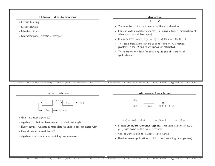
optimum filter applications introduction rc o d inverse
play

Optimum Filter Applications Introduction Rc o = d Inverse filtering - PowerPoint PPT Presentation

Optimum Filter Applications Introduction Rc o = d Inverse filtering You now know the basic model for linear estimation Deconvolution Can estimate a random variable y ( n ) using a linear combination of Matched filters other


  1. Optimum Filter Applications Introduction Rc o = d • Inverse filtering • You now know the basic model for linear estimation • Deconvolution • Can estimate a random variable y ( n ) using a linear combination of • Matched filters other random variables x i ( n ) • Microelectrode Detection Example • In our context, often x i ( n ) = x ( n − i ) for i = 0 to M − 1 • The basic framework can be used to solve many practical problems, once R and d are known or estimated • There are many tricks for obtaining R and d in practical applications J. McNames Portland State University ECE 539/639 Applications Ver. 1.02 1 J. McNames Portland State University ECE 539/639 Applications Ver. 1.02 2 Signal Prediction Interference Cancellation y ( n ) x ( n − L ) ˆ x ( n ) z − L x ( n ) ˆ H ( z ) − ˆ x ( n ) � e ( n ) H ( z ) ˆ x ( n + L ) ˆ H ( z ) • Goal: estimate x ( n + L ) y ( n ) = s ( n ) + v ( n ) r xv ( ℓ ) � = 0 r xs ( ℓ ) = 0 • Application that we have already studied and applied • If x ( n ) are noise reference signals , then e ( n ) is an estimate of • Every sample, we obtain more data to update our estimator with y ( n ) with some of the noise removed • How do we do so efficiently? • Can be generalized to multiple input signals • Applications: prediction, modeling, compression • Used in many applications (think noise cancelling head phones) J. McNames Portland State University ECE 539/639 Applications Ver. 1.02 3 J. McNames Portland State University ECE 539/639 Applications Ver. 1.02 4

  2. System Identification System Inversion v ( n ) v ( n ) x ( n ) x ( n ) H ( z ) � y ( n ) H − 1 ( z ) ˆ y ( n ) H ( z ) � ˆ y ( n ) ˆ y ( n ) ˆ H ( z ) • Know as inverse system modeling , inverse filtering , • Know as system modeling deconvolution • If we can stimulate the system under normal operating conditions, • Goal: estimate an inverse of the system we can estimate r x ( ℓ ) and r yx ( ℓ ) • Useful for adaptive equalization, deconvolution, and adaptive • In this case ˆ H ( z ) could be an PZ system, since both the input inverse control and the output are observable • Still requires r x ( ℓ ) and r yx ( ℓ ) • What good is ˆ H ( z ) ? • Applications include echo cancelation, channel modeling, and system identification J. McNames Portland State University ECE 539/639 Applications Ver. 1.02 5 J. McNames Portland State University ECE 539/639 Applications Ver. 1.02 6 Blind Deconvolution Optimum Inverse Modeling x ( n ) v ( n ) w ( n ) G ( z ) H ( z ) y ( n ) x ( n ) y ( n ) G ( z ) � H ( z ) y ( n ) ˆ • In this case the input is unknown as well as the system G ( z ) • Goal is to estimate the (possibly delayed and scaled) input w ( n ) • Ideally we would like to obtain y ( n ) from x ( n ) and possibly the system • May be difficult if h ( n ) ∗ g ( n ) ∗ w ( n ) ≈ b 0 w ( n − n 0 ) – G ( z ) contains a delay h ( n ) ∗ g ( n ) ≈ b 0 δ ( n − n 0 ) – The additive noise is significant • Problem is ill-defined if we have no information about w ( n ) – G ( z ) is nonminimum phase – The inverse system is IIR • Need to know something about • In practice, H ( z ) is an FIR filter r xy ( ℓ ) = r xw ( ℓ ) = g ( ℓ ) ∗ r w ( ℓ ) • In some applications a delayed estimate is acceptable, • Often assume w ( n ) is a WN(0 , σ 2 w ) process y ( n ) = ≈ y ( n − D ) ˆ J. McNames Portland State University ECE 539/639 Applications Ver. 1.02 7 J. McNames Portland State University ECE 539/639 Applications Ver. 1.02 8

  3. Remaining Tasks Matched Filters: Problem Definition M × 1 ( n ) = s ( n ) + v ( n ) x • Add an example with a synthetic signal and known system much like Example 6.7.1 in the text where s ( n ) is the signal of interest and v ( n ) is a noise signal • Add a practical example • Suppose we have “brief” events of interest that occur in a noisy background • Goal: detect the events • Applications: radar, sonar, microelectrode recordings, communications • Suppose we decide to form a linear combination, y ( n ) = c H x ( n ) and then apply a threshold for detection • Generally it is assumed that R s i ( ℓ ) = σ 2 R v j ( ℓ ) = σ 2 s i δ ( ℓ ) ∀ i v j δ ( ℓ ) ∀ j R s i v j ( ℓ ) = 0 J. McNames Portland State University ECE 539/639 Applications Ver. 1.02 9 J. McNames Portland State University ECE 539/639 Applications Ver. 1.02 10 Matched Filters: Estimator Properties Matched Filters: Detection Metrics Events Non-events y ( n ) = c H x ( n ) = c H s ( n ) + c H v ( n ) Detected TP FP N D � | y ( n ) | 2 � � c H x ( n ) x H ( n ) c � = c H R x ( n ) c P y ( n ) = E = E Not detected FN TN N ¯ D N E N ¯ E • The output power depends only on the signal autocorrelation matrix TP TP • Sensitivity : N E = TP+FN – Fraction of events that are detected • Because s ( n ) ⊥ v ( n ) , R x ( n ) can be expressed as TN TN • Specificity : E = x ( n ) x H ( n ) � � R x ( n ) = E N ¯ FP+TN – Fraction of non-events that are not detected � ( s ( n ) + v ( n )) ( s ( n ) + v ( n )) H � = E TP TP • Positive Predictivity : N D = TP+FP s ( n ) s H ( n ) v ( n ) v H ( n ) � � � � = E + E – Fraction of detected events that are events = R s ( n ) + R v ( n ) TN TN • Negative Predictivity : D = N ¯ FN+TN Signal Power Noise Power – Fraction of nondetected events that are not events • The structure of R s ( n ) depends on the statistical model of s ( n ) J. McNames Portland State University ECE 539/639 Applications Ver. 1.02 11 J. McNames Portland State University ECE 539/639 Applications Ver. 1.02 12

  4. Matched Filters: Metric Selection Matched Filters: Signal-to-Noise Ratio • Goal: maximize the detection accuracy y ( n ) = c H x ( n ) = c H s ( n ) c H v ( n ) – Minimize the number of false positives and false negatives P y ( n ) = c H R x ( n ) c = c H R s ( n ) c + c H R v ( n ) c – Maximize the sensitivity and specificity – Maximize the positive predictivity and negative predictivity • Proxy goal: Find c such that the signal-to-noise ratio is maximized • There is almost always a tradeoff between each of these pairs SNR = c H R s ( n ) c • Threshold controls the tradeoff c H R v ( n ) c • For a given tradeoff, what is the best parameter vector c ? • Rationale: detection will be easier if • Relationship is difficult to obtain in general – y ( n ) is large when signal is present – y ( n ) is small when only noise is present J. McNames Portland State University ECE 539/639 Applications Ver. 1.02 13 J. McNames Portland State University ECE 539/639 Applications Ver. 1.02 14 Matched Filters: Problem Classes Matched Filters: Deterministic Signal in White Noise x ( n ) = s ( n ) + v ( n ) s ( n ) = α s 0 • The signal may be | c H α s 0 | 2 � = P α | c H s 0 | 2 � P s ( n ) = E – Random with autocorrelation matrix R s ( n ) | c H s 0 | 2 – Deterministic with random amplitude, s ( n ) = α s 0 SNR( c ) = P α c H R v c • Similarly, the noise may be colored or white Now if R v ( n ) = σ 2 v I • Four problems altogether | c H s 0 | 2 SNR( c ) = P α • Consider one at a time c H c P v From the Cauchy-Schwartz inequality � c H s 0 ≤ ( c H c )( s H 0 s 0 ) | c H s 0 | 2 ( c H c )( s H SNR( c ) = P α ≤ P α 0 s 0 ) = P α s H 0 s 0 c H c c H c P v P v P v J. McNames Portland State University ECE 539/639 Applications Ver. 1.02 15 J. McNames Portland State University ECE 539/639 Applications Ver. 1.02 16

  5. Matched Filters: Deterministic Signal in White Noise Matched Filters: Deterministic Signal in Colored Noise If the noise covariance matrix R v ( n ) is positive definite, then there SNR o ( c ) = P α s H c o = β s 0 0 s 0 exists a square root such that P v R v = L v L H • The SNR is maximized when c is the same as the expected event v shape • The text assumes that L v is a lower-upper Cholesky • This is why it is called a matched filter decomposition, but it could be any square root of R v ( n ) for this application • SNR is scale invariant SNR( c ) = SNR( β c ) • Here I am assuming the signal and noise are jointly stationary to simplify notation, but it works in the nonstationary case as well J. McNames Portland State University ECE 539/639 Applications Ver. 1.02 17 J. McNames Portland State University ECE 539/639 Applications Ver. 1.02 18 Matched Filters: Whitening Matched Filters: Colored Noise SNR Let us define | c H s 0 | 2 | c H L v L − 1 v s 0 | 2 SNR( c ) = P α = P α v ( n ) � L − 1 c H R v c c H L v L H v c ˜ v v ( n ) | ( L H v c ) H ( L − 1 v s 0 ) | 2 c H ˜ s 0 ) | 2 | ˜ ( L − 1 v v ( n ))( L − 1 v v ( n )) H � � R ˜ v = E = P α = P α ( L H v c ) H ( L H c H ˜ v c ) ˜ c L − 1 v v ( n ) v H ( n ) L − H � � = E v where = L − 1 v ( n ) v H ( n ) L − H � � v E v c � L H s 0 � L − 1 ˜ ˜ v c v s 0 = L − 1 v R v L − H ( n ) v = L − 1 v L v L H v L − H ( n ) Thus, this reduces to the same problem as the white noise case and v the solution follows immediately = I c o = β L − H L − 1 v s 0 = β R − 1 c o = β ˜ ˜ s 0 v s 0 v SNR o ( c ) = P α SNR o ( c ) = P α s H s H 0 R − 1 ˜ 0 ˜ s 0 v s 0 P v P v J. McNames Portland State University ECE 539/639 Applications Ver. 1.02 19 J. McNames Portland State University ECE 539/639 Applications Ver. 1.02 20

Download Presentation
Download Policy: The content available on the website is offered to you 'AS IS' for your personal information and use only. It cannot be commercialized, licensed, or distributed on other websites without prior consent from the author. To download a presentation, simply click this link. If you encounter any difficulties during the download process, it's possible that the publisher has removed the file from their server.

Recommend


More recommend