Optimizing the Inner Loop of the Gravitational Force Interaction on - - PowerPoint PPT Presentation

▶

Jul 05, 2023 138 likes •351 views

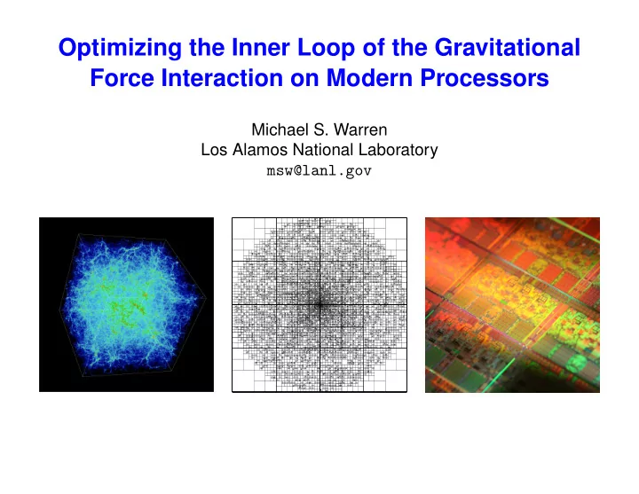
Optimizing the Inner Loop of the Gravitational Force Interaction on Modern Processors Michael S. Warren Los Alamos National Laboratory msw@lanl.gov Gravitational Force r i r j F i = GM i M j 3 r j || 2 + 2 ) 2 ( ||

SLIDE 1

Optimizing the Inner Loop of the Gravitational Force Interaction on Modern Processors

Michael S. Warren Los Alamos National Laboratory msw@lanl.gov

SLIDE 2

Gravitational Force

Fi = GMi
0≤j=i<N

Mj

ri −

rj (|| ri − rj||2 + ǫ2)

3 2

Figure 1: The Gravitational N-body Problem

SLIDE 3

Inner Loop Performance

Processor libm Karp 40-MHz Intel i860 35.2 167-MHz Cray Y-MP (est) 50.0 500-MHz Intel P3 87.6 185.6 533-MHz Alpha EV56 76.2 242.2 933-MHz Transmeta TM5800 189.5 373.2 375-MHz IBM Power3 298.5 514.4 1133-MHz Intel P3 292.2 594.9 1200-MHz AMD Athlon MP 350.7 614.0 1800-MHz AMD Athlon XP 609.9 951.9 1250-MHz Alpha 21264C 935.2 1141.0 2530-MHz Intel P4 (icc) 1170.0 1357.0 2530-MHz Intel P4 (SSE) 6514.0 2600-MHz AMD Opteron (SSE3) 7380.0 2600-MHz AMD Opteron 8435 13878.0 2660-MHz Intel Xeon E5430 16343.0 PowerXCell 8i (single SPE) 16356.0 Table 1: Mflop/s obtained on our gravitational micro-kernel benchmark.

SLIDE 4

Should we Optimize?

“We should forget about small efficiencies, say about 97% of the time: premature

ptimization is the root of all evil.”

—Donald Knuth

SLIDE 5

What is Most Important to Optimize?

Figure 2: Representative fractions of time spent in phases of parallel code

SLIDE 6

Can you outrun Moore’s Law?

Figure 3: Intel CPU Introductions (Herb Sutter)

SLIDE 7

Where are we?

Figure 4: Gartner Hype Cycle

SLIDE 8

Current CPU Trends

Figure 5: PetaFLOPS for the Common Man (Jeff Layton, Dell)

SLIDE 9

Specific Issues

Vectorization (SIMD)
Instruction Latency (pipelining)
Reciprocal Square Root (Newton-Raphson if necessary)
Memory Bandwidth (Kills co-processor approach)
Available registers (Limits concurrency)
Swizzling (Data Layout)
Portability/Libraries (Learn from BLAS/Automatic Tuning?)

SLIDE 10

SSE3 Code for Inner Loop

112 flops in 38 cycles, 11 add/sub, 9 mul, 1 rsqrt

loop: movaps (%rdi), %xmm0 # mass rsqrtps %xmm4, %xmm4 movaps 16(%rdi), %xmm5 # x movaps %xmm0, %xmm1 movaps 32(%rdi), %xmm6 # y addps %xmm1, %xmm11 # mass movaps 48(%rdi), %xmm7 # z addq $64, %rdi subps %xmm8, %xmm5 cmpq %rsi, %rdi subps %xmm9, %xmm6 mulps %xmm4, %xmm0 subps %xmm10, %xmm7 mulps %xmm4, %xmm4 movaps %xmm5, %xmm1 mulps %xmm0, %xmm4 movaps %xmm6, %xmm2 addps %xmm0, %xmm12 # phi movaps %xmm7, %xmm3 mulps %xmm4, %xmm5 movaps (%rsp), %xmm4 # eps mulps %xmm4, %xmm6 mulps %xmm1, %xmm1 mulps %xmm4, %xmm7 mulps %xmm2, %xmm2 addps %xmm5, %xmm13 # ax mulps %xmm3, %xmm3 addps %xmm6, %xmm14 # ay addps %xmm1, %xmm4 addps %xmm7, %xmm15 # az jb .loop # Prob 97% addps %xmm2, %xmm4 addps %xmm3, %xmm4

SLIDE 11

Specific Issues

Vectorization (SIMD)
Instruction Latency (pipelining)
Reciprocal Square Root (Newton-Raphson if necessary)
Memory Bandwidth (Kills co-processor approach)
Available registers (Limits concurrency)
Swizzling (Data Layout)
Portability/Libraries (Learn from BLAS/Automatic Tuning?)

SLIDE 12

Pipelines

Figure 6: Instruction Pipelining (Wikipedia)

SLIDE 13

Cell Code for Inner Loop

/* Need to unroll by pipeline depth (6) for optimal performance */

for (i = 0; i <= n/16; i++) { mass = *(vector float *)p; dx = *(vector float *)(p+4); dy = *(vector float *)(p+8); dz = *(vector float *)(p+12); dx = spu_sub(dx, pposx); dy = spu_sub(dy, pposy); dz = spu_sub(dz, pposz); dr2 = spu_madd(dx, dx, eps2); dr2 = spu_madd(dy, dy, dr2); dr2 = spu_madd(dz, dz, dr2); phii = spu_rsqrte(dr2); mor3 = spu_mul(phii, phii); phii = spu_mul(phii, mass); total_mass = spu_add(total_mass, mass); p += 16; mor3 = spu_mul(mor3, phii); phi = spu_sub(phi, phii); ax = spu_madd(mor3, dx, ax); ay = spu_madd(mor3, dy, ay); az = spu_madd(mor3, dz, az); }

SLIDE 14

Specific Issues

Vectorization (SIMD)
Instruction Latency (pipelining)
Reciprocal Square Root (Newton-Raphson if necessary)
Memory Bandwidth (Kills co-processor approach)
Available registers (Limits concurrency)
Swizzling (Data Layout)
Portability/Libraries (Learn from BLAS/Automatic Tuning?)

SLIDE 15

i860 Assembly Code

frsqr.ss g0, t0 // initial guess of inverse sqrt pfmul.ss t2, t3, f0 frsqr.ss g1, t1 pfmul.ss g0, t0, t0 // (0.5 * x) * yold frsqr.ss g2, t2 pfmul.ss g1, t1, t1 pfmul.ss c2, g0, f0 // 0.5 * x pfmul.ss g2, t2, t2 pfmul.ss c2, g1, f0 pfmul.ss t0, t3, t3 // yold * ( ) pfmul.ss c2, g2, f0 pfmul.ss t1, t3, t3 pfmul.ss t0, t0, g0 // yold * yold pfmul.ss t2, t3, t3 pfmul.ss t1, t1, g1 mr2s1.ss c1, f0, f0 // 1.5 - ( ) pfmul.ss t2, t2, g2 mr2s1.ss c1, f0, f0 pfmul.ss g0, t3, t3 // (0.5 * x) * (yold * yold) mr2s1.ss c1, f0, f0 pfmul.ss g1, t3, t3 pfadd.ss f0, f0, t3 pfmul.ss g2, t3, t3 pfmul.ss t0, t3, f0 // yold * ( ) mr2s1.ss c1, f0, f0 // 1.5 - ( ) pfadd.ss f0, f0, t3 mr2s1.ss c1, f0, f0 pfmul.ss t1, t3, f0 mr2s1.ss c1, f0, f0 pfadd.ss f0, f0, t3 pfadd.ss f0, f0, t3 pfmul.ss t2, t3, f0 pfmul.ss t0, t3, f0 // yold * ( ) pfmul.ss f0, f0, g0 // result pfadd.ss f0, f0, t3 pfmul.ss f0, f0, g1 pfmul.ss t1, t3, f0 pfmul.ss f0, f0, g2 pfadd.ss f0, f0, t3

SLIDE 16

Specific Issues

Vectorization (SIMD)
Instruction Latency (pipelining)
Reciprocal Square Root (Newton-Raphson if necessary)
Memory Bandwidth (Kills co-processor approach)
Available registers (Limits concurrency)
Swizzling (Data Layout)
Portability/Libraries (Learn from BLAS/Automatic Tuning?)

SLIDE 17

Memory Bandwidth “Those who cannot remember the past are condemned to repeat it.” —George Santayana

/* Copy Data for CM-5 Vector Unit */ bodies = (aux float *)aux_alloc_heap(n); for (j = 0; j < cnt/(4*VLEN*N_DP); j++) { for (i = 0; i < N_DP; i++) { dp_copy((double *)(p+(i+j*N_DP)*4*VLEN), (double *)(p+(i+1+j*N_DP)*4*VLEN), (aux double *)(bodies+(last_icnt*4/N_DP)+j*4*VLEN), dp[i]); } } bodies = AC_change_dp(bodies, ALL_DPS); do_grav_vu(bodies, bodies+n/N_DP, pos0, &mass, acc, &phi, eps2p);

The gravitational inner loop requires approximately 1 byte/sec of bandwidth for each floating point operation per second. e.g. a Cell QS22 blade requires 256 Gbytes/sec, a Tesla C1060 requires 512 Gbytes/sec. PCI-Express x16 provides 3.2 Gbytes/sec.

SLIDE 18

Specific Issues

Vectorization (SIMD)
Instruction Latency (pipelining)
Reciprocal Square Root (Newton-Raphson if necessary)
Memory Bandwidth (Kills co-processor approach)
Available registers (Limits concurrency)
Swizzling (Data Layout)
Portability/Libraries (Learn from BLAS/Automatic Tuning?)

SLIDE 19

Specific Issues

Vectorization (SIMD)
Instruction Latency (pipelining)
Reciprocal Square Root (Newton-Raphson if necessary)
Memory Bandwidth (Kills co-processor approach)
Available registers (Limits concurrency)
Swizzling (Data Layout)
Portability/Libraries (Learn from BLAS/Automatic Tuning?)

SLIDE 20

Specific Issues

Vectorization (SIMD)
Instruction Latency (pipelining)
Reciprocal Square Root (Newton-Raphson if necessary)
Memory Bandwidth (Kills co-processor approach)
Available registers (Limits concurrency)
Swizzling (Data Layout)
Portability/Libraries (Learn from BLAS/Automatic Tuning?)

SLIDE 21

Historical Treecode Performance

Year Site Machine Procs Gflop/s Mflops/proc 2006 LANL Coyote (SSE3) 448 1880 4200.0 2004 LANL Space Simulator (SSE) 288 1166 4050.0 2003 LANL ASCI QB 3600 2793 775.8 2002 NERSC IBM SP-3(375/W) 256 57.70 225.0 2000 LANL SGI Origin 2000 64 13.10 205.0 1996 Sandia ASCI Red 6800 464.9 68.4 1995 JPL Cray T3D 256 7.94 31.0 1995 LANL TMC CM-5 512 14.06 27.5 1993 Caltech Intel Delta 512 10.02 19.6 Table 2: Performance of HOT on a variety of parallel supercomputers.