Operational Semantics This course Why semantics? y := 1; precise - - PowerPoint PPT Presentation

This course Why semantics?

• precise specification of software and

hardware

• facilitate reasoning about systems:

testing may reveal errors but not their absense

• form the basis for prototype imple-

mentations, e.g. interpreters and com- pilers Why functional programming?

• based on mathematical notation, not
• n the von Neuman architecture
• excelent for prototype definitions

I.1

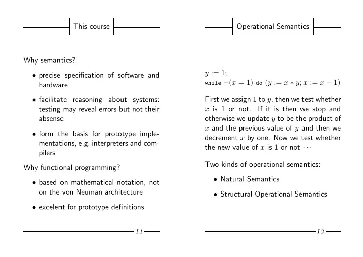
Operational Semantics y := 1;

while ¬(x = 1) do (y := x ∗ y; x := x − 1)

First we assign 1 to y, then we test whether x is 1 or not. If it is then we stop and

• therwise we update y to be the product of

x and the previous value of y and then we decrement x by one. Now we test whether the new value of x is 1 or not · · · Two kinds of operational semantics:

• Natural Semantics
• Structural Operational Semantics

I.2

Denotational Semantics y := 1;

while ¬(x = 1) do (y := x ∗ y; x := x − 1)

The program computes a partial function from states to states: the final state will be equal to the initial state except that the value of x will be 1 and the value of y will be equal to the factorial of the value of x in the initial state. Two kinds of denotational semantics:

• Direct Style Semantics
• Continuation Style Semantics

I.3

Axiomatic Semantics y := 1;

while ¬(x = 1) do (y := x ∗ y; x := x − 1)

If x = n holds before the program is exe- cuted then y = n! will hold when the exe- cution terminates (if it terminates) Two kinds of axiomatic semantics:

• Partial Correctness
• Total Correctness

I.4

Which approach? Programming Language

↓

Semantics

• natural semantics
• structural operational semantics
• direct style denotational semantics
• continuation style denotational se-

mantics

• partial correctness axiomatic seman-

tics

• total correctness axiomatic semantics

I.5

Selection criteria

• constructs of the language

– imperative – functional – concurrent/parallel – object oriented – non-deterministic – · · ·

• what is the semantics used for

– understanding the language – verification of programs – prototyping – compiler construction – program analysis – · · ·

I.6

While language Theoretical Development S ::= x := a | skip | S1; S2 | if b then S1 else S2 | while b do S | repeat S until b natural semantics

• struct. op.

semantics direct style

• den. sem.
• cont. style
• den. sem.

partial correctness total correctness

I.7

Approach concrete LL(1)/LALR(1) grammar syntax concrete syntax trees ↓ abstract syntactic categories syntax abstract syntax trees ↓ semantics semantic categories semantic definitions

I.8

Miranda Programming languages

• imperative (procedural)
• applicative (functional)

– lazy languages Miranda – eager languages Standard ML Lisp?, Scheme?

• declarative (logical)
• object-oriented
• concurrent / parallel
• · · ·

I.9

Syntactic Categories for While language

• numerals

n ∈ Num

• variables

x ∈ Var

• arithmetic expressions

a ∈ Aexp a ::= n | x | a1 + a2 | a1 ∗ a2 | a1 − a2

• booleans expressions

b ∈ Bexp b ::= true | false | a1 = a2 | a1 ≤ a2 | ¬ b | b1 ∧ b2

• statements

S ∈ Stm S ::= x := a | skip | S1; S2 | if b then S1 else S2 | while b do S

II.1

Semantic Categories Natural numbers N = {0, 1, 2, · · ·} Truth values T = {tt, ff} States

• State = Var → N
• State′ = (Var × N)∗
• State′′ = Var∗ × N∗

Lookup in a state: s x Update a state: s′ = s[y → v] s′ x =

  

s x if x = y v if x = y

II.2

Meanings of the syntactic categories Numerals N : Num → N Variables s ∈ State = Var → N Arithmetic expressions A : Aexp → (State → N) Boolean expressions B : Bexp → (State → T) Statements S : Stm → (State ֒ → State)

II.3

A : Aexp → State → N A[n]s = N[n] A[x]s = s x A[a1 + a2]s = A[a1]s + A[a2]s A[a1 ∗ a2]s = A[a1]s ∗ A[a2]s A[a1 − a2]s = A[a1]s − A[a2]s

II.4

B : Bexp → State → T B[true]s = tt B[false]s = ff B[a1 = a2]s =

    

tt if A[a1]s = A[a2]s ff if A[a1]s = A[a2]s B[a1 ≤ a2]s =

    

tt if A[a1]s ≤ A[a2]s ff if A[a1]s ≤ A[a2]s B[¬b]s =

    

tt if B[b]s = ff ff if B[b]s = tt B[b1 ∧ b2]s =

                

tt if B[b1]s = tt and B[b2]s = tt ff if B[b1]s = ff

• r B[b2]s = ff

II.5

Compositional Definitions

• The syntactic categories are specified

by an abstract syntax giving a unique decomposition of each element into its constituents.

• The semantics is defined by composi-

tional definitions of functions. Since the decomposition of the ele- ments is unique this means that the semantics is well-defined.

II.6

Statements Syntactic Category S ::= x := a | skip | S1; S2 | if b then S1 else S2 | while b do S Meaning of the syntactic category: S : Stm → (State ֒ → State) Two operational semantics

• Natural Semantics
• Structural Operational Semantics

specified by transition systems

II.7

Transition System (Γ, T, >)

• Γ: a set of configurations
• T: a set of terminal configurations

T ⊆ Γ

• >: a transition relation

> ⊆ Γ × Γ

II.8

Natural semantics Idea: describe how the overall result of the computation is obtained Transition system: (Γ, T, →)

• Γ = {(S, s) | S ∈ While, s ∈ State}

∪ State

• T = State
• → ⊆ {(S, s) | S ∈ While, s ∈ State}

× State Typical transition: (S, s) → s′ where S is the program s is the initial state s′ is the final state

II.9

Natural Semantics (x := a, s) → s[x → A[a]s] (skip, s) → s (S1, s) → s′, (S2, s′) → s′′ (S1; S2, s) → s′′ (S1, s) → s′ (if b then S1 else S2, s) → s′ if B[b]s = tt (S2, s) → s′ (if b then S1 else S2, s) → s′ if B[b]s = ff (S, s) → s′, (while b do S, s′) → s′′ (while b do S, s) → s′′ if B[b]s = tt (while b do S, s) → s if B[b]s = ff

II.10