ONE WAY TO DESIGN THE CONTROL LAW OF A MINI-UAV Projet c o l e - - PowerPoint PPT Presentation

one way to design the control law of a mini uav
SMART_READER_LITE
LIVE PREVIEW

ONE WAY TO DESIGN THE CONTROL LAW OF A MINI-UAV Projet c o l e - - PowerPoint PPT Presentation

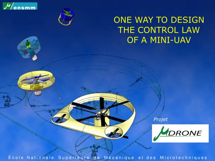
ONE WAY TO DESIGN THE CONTROL LAW OF A MINI-UAV Projet c o l e N a t i o n a l e S u p r i e u r e d e M c a n i q u e e t d e s M i c r o t e c h n i q u e s Plan Introduction Model of the Drone


slide-1
SLIDE 1

É c o l e N a t i o n a l e S u p é r i e u r e d e M é c a n i q u e e t d e s M i c r o t e c h n i q u e s

ONE WAY TO DESIGN THE CONTROL LAW OF A MINI-UAV

Projet

slide-2
SLIDE 2

É c o l e N a t i o n a l e S u p é r i e u r e d e M é c a n i q u e e t d e s M i c r o t e c h n i q u e s

 Plan

  • Introduction
  • Model of the μDrone
  • Control design of the MAV
  • Choice of the adjustment parameters
  • Conclusion
slide-3
SLIDE 3

É c o l e N a t i o n a l e S u p é r i e u r e d e M é c a n i q u e e t d e s M i c r o t e c h n i q u e s

 Introduction

  • The ENSMM μDrone

This MAV uses six propellers to fly :

  • Two are counter-rotating and provide the lift
  • Two provide the trim stabilization
  • Two are used for the propulsion
  • Approximation of the MAV behaviour

The model is a MIMO linear time-invariant system

  • Control design of the MAV

The LQ state feedback regulator design is applied to a « standard model » To compute the weighting matrices of quadratic criterions we use a « partial observability gramian »

The great advantage of this method is due to the use of only three scalars to synthesize a robust control law.

slide-4
SLIDE 4

É c o l e N a t i o n a l e S u p é r i e u r e d e M é c a n i q u e e t d e s M i c r o t e c h n i q u e s

 Model of the μDrone

The μDrone is a « gyrodyne » with six propellers We worked on the assumption that it can be described as seven solids in interaction

  • Model of the actuators

Let denote the thrust produced by the ith actuator and the associated

  • moment. If denotes the control input of the actuator, we assume that
  • Global model

With this assumption and after linearization of the mecanical model in the vicinity of a horizontal trim, the following MIMO linear time-invariant system is an approximation of the MAV behaviour :

i

F

i

M

i

u

slide-5
SLIDE 5

É c o l e N a t i o n a l e S u p é r i e u r e d e M é c a n i q u e e t d e s M i c r o t e c h n i q u e s

 Control design of the MAV

  • Standard model

We introduce a constant perturbation vector : Initial model is then augmented :

  • Extraction of an observable subsystem
slide-6
SLIDE 6

É c o l e N a t i o n a l e S u p é r i e u r e d e M é c a n i q u e e t d e s M i c r o t e c h n i q u e s

  • k
  • State estimator
  • Gain matrix is chosen as the solution of the LQ problem :

A positive scalar is to be designed so that and the weighting matrices where is a partial observability gramian

  • k
slide-7
SLIDE 7

É c o l e N a t i o n a l e S u p é r i e u r e d e M é c a n i q u e e t d e s M i c r o t e c h n i q u e s

Partial observability gramian :

where

State estimator is then :

slide-8
SLIDE 8

É c o l e N a t i o n a l e S u p é r i e u r e d e M é c a n i q u e e t d e s M i c r o t e c h n i q u e s

  • Uncontrollable modes influence rejection
  • Controllability staircase form of

uncontrollable modes perturb controllable ones

  • Rejection with a linear transformation

leading to :

nc

x

slide-9
SLIDE 9

É c o l e N a t i o n a l e S u p é r i e u r e d e M é c a n i q u e e t d e s M i c r o t e c h n i q u e s

It is often possible to find such as : with these conditions :

A state feedback is then possible…

slide-10
SLIDE 10

É c o l e N a t i o n a l e S u p é r i e u r e d e M é c a n i q u e e t d e s M i c r o t e c h n i q u e s

  • Control feedback
  • New LQ problem

choice of the weighting matrices

define another positive scalar , a positive control horizon such as : and the partial observability gramian :

c

k

c

T

slide-11
SLIDE 11

É c o l e N a t i o n a l e S u p é r i e u r e d e M é c a n i q u e e t d e s M i c r o t e c h n i q u e s

  • Feedback control elaboration

with this feedback control the system is : and we want at permanent rate : If that matrix is invertible, the solution is :

slide-12
SLIDE 12

É c o l e N a t i o n a l e S u p é r i e u r e d e M é c a n i q u e e t d e s M i c r o t e c h n i q u e s

Then, the control vector is : and the use of transformation matrix leads to

  • Regulator equations

with

  • c

T

slide-13
SLIDE 13

É c o l e N a t i o n a l e S u p é r i e u r e d e M é c a n i q u e e t d e s M i c r o t e c h n i q u e s

 Choice of the adjustment parameters

  • First step

Assign a fixed value to

,

Adjust filtering horizon so that is a stability matrix.

  • Second step (quantify the stability robustness)

The regulator, without reference, is converted to a transfer matrix with

  • T

reg

A

slide-14
SLIDE 14

É c o l e N a t i o n a l e S u p é r i e u r e d e M é c a n i q u e e t d e s M i c r o t e c h n i q u e s

  • Similarly, initial model of the MAV is converted to
  • Now define
  • Loop transfers
  • Static margin
  • Dynamic margin
  • When is a stability matrix, feedback is robust in relation to :

and

reg

A

slide-15
SLIDE 15

É c o l e N a t i o n a l e S u p é r i e u r e d e M é c a n i q u e e t d e s M i c r o t e c h n i q u e s

  • Last step

Now it is not difficult to compute static and dynamic margins for different values of the three parameters :

  • Filtering horizon
  • Shape factor
  • Recovery factor

The reasons why this strategy is often efficient is due to :

  • The natural robustness of a LQ problem solution
  • The notion of loop transfer recovery (LTR)
  • T
  • k

c

k

slide-16
SLIDE 16

É c o l e N a t i o n a l e S u p é r i e u r e d e M é c a n i q u e e t d e s M i c r o t e c h n i q u e s

  • Implementation on the μDrone

Static margin : Dynamic margin :

1.2

  • T

s

1.2

  • k

3.2

c

k

42.2%

st

M 32.7

dyn

M ms

slide-17
SLIDE 17

É c o l e N a t i o n a l e S u p é r i e u r e d e M é c a n i q u e e t d e s M i c r o t e c h n i q u e s

slide-18
SLIDE 18

É c o l e N a t i o n a l e S u p é r i e u r e d e M é c a n i q u e e t d e s M i c r o t e c h n i q u e s

 Conclusion

  • The proposed method is quite easy to use

Only three positive scalars have to be adjusted

  • Tricky problems

Rejection of uncontrollable modes is not always possible Internal stability of regulator is sometimes difficult to reach

  • Philippe de Larminat’s recent book in which this method is

explained in detail is of great interest.