off the the shelf classifiers shelf classifiers off
play

Off- -The The- -Shelf Classifiers Shelf Classifiers Off A - PowerPoint PPT Presentation

Off- -The The- -Shelf Classifiers Shelf Classifiers Off A method that can be applied directly to A method that can be applied directly to data without requiring a great deal of time- - data without requiring a great deal of time consuming


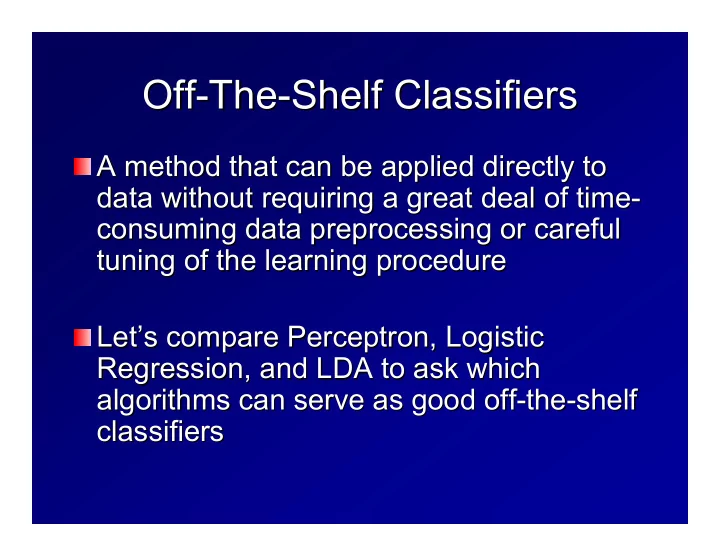
  1. Off- -The The- -Shelf Classifiers Shelf Classifiers Off A method that can be applied directly to A method that can be applied directly to data without requiring a great deal of time- - data without requiring a great deal of time consuming data preprocessing or careful consuming data preprocessing or careful tuning of the learning procedure tuning of the learning procedure Let’ ’s compare Perceptron, Logistic s compare Perceptron, Logistic Let Regression, and LDA to ask which Regression, and LDA to ask which algorithms can serve as good off- -the the- -shelf shelf algorithms can serve as good off classifiers classifiers

  2. Off- -The The- -Shelf Criteria Shelf Criteria Off Natural handling of “ “mixed mixed” ” data types data types Natural handling of – continuous, ordered continuous, ordered- -discrete, unordered discrete, unordered- -discrete discrete – Handling of missing values Handling of missing values Robustness to outliers in input space Robustness to outliers in input space Insensitive to monotone transformations of input features Insensitive to monotone transformations of input features Computational scalability for large data sets Computational scalability for large data sets Ability to deal with irrelevant inputs Ability to deal with irrelevant inputs Ability to extract linear combinations of features Ability to extract linear combinations of features Interpretability Interpretability Predictive power Predictive power

  3. Handling Mixed Data Types with Handling Mixed Data Types with Numerical Classifiers Numerical Classifiers Indicator Variables Indicator Variables – sex: Convert to 0/1 variable sex: Convert to 0/1 variable – – county county- -of of- -residence: Introduce a 0/1 variable for each residence: Introduce a 0/1 variable for each – county county Ordered- -discrete variables discrete variables Ordered – example: {small, medium, large} example: {small, medium, large} – – Treat as unordered Treat as unordered – – Treat as real Treat as real- -valued valued – Sometimes it is possible to measure the “ Sometimes it is possible to measure the “distance distance” ” between between discrete terms. For example, how often is one value discrete terms. For example, how often is one value mistaken for another? These distances can then be mistaken for another? These distances can then be combined via multi- -dimensional scaling to assign real values dimensional scaling to assign real values combined via multi

  4. Missing Values Missing Values Two basic causes of missing values Two basic causes of missing values – Missing at random: independent errors cause Missing at random: independent errors cause – features to be missing. Examples: features to be missing. Examples: clouds prevent satellite from seeing the ground. clouds prevent satellite from seeing the ground. data transmission (wireless network) is lost from time- -to to- -time time data transmission (wireless network) is lost from time – Missing for cause: Missing for cause: – Results of a medical test are missing because physician Results of a medical test are missing because physician decided not to perform it. decided not to perform it. Very large or very small values fail to be recorded Very large or very small values fail to be recorded Human subjects refuse to answer personal questions Human subjects refuse to answer personal questions

  5. Dealing with Missing Values Dealing with Missing Values Missing at Random Missing at Random – P( P( x , y ) methods can still learn a model of P( x ), even when some – x , y ) methods can still learn a model of P( x ), even when some features are not measured. features are not measured. – The EM algorithm can be applied to fill in th emissing features The EM algorithm can be applied to fill in th emissing features with the with the – most likely values for those features most likely values for those features – A simpler approach is to replace each missing value by its avera A simpler approach is to replace each missing value by its average ge – value or its most likely value value or its most likely value – There are specialized methods for decision trees There are specialized methods for decision trees – Missing for cause Missing for cause – The – The “ “first principles first principles” ” approach is to model the causes of the missing approach is to model the causes of the missing data as additional hidden variables and then try to fit the combined ined data as additional hidden variables and then try to fit the comb model to the available data. model to the available data. – Another approach is to treat Another approach is to treat “ “missing missing” ” as a separate value for the as a separate value for the – feature feature For discrete features, this is easy For discrete features, this is easy For continuous features, we typically introduce an indicator fea For continuous features, we typically introduce an indicator feature that is 1 ture that is 1 if the associated real- -valued feature was observed and 0 if not. valued feature was observed and 0 if not. if the associated real

  6. Robust to Outliers in the Input Robust to Outliers in the Input Space Space Perceptron: Outliers can cause the Perceptron: Outliers can cause the algorithm to loop forever algorithm to loop forever Logistic Regression: Outliers far from the Logistic Regression: Outliers far from the decision boundary have little impact – – decision boundary have little impact robust! robust! LDA/QDA: Outliers have a strong impact LDA/QDA: Outliers have a strong impact on the models of P( x | y ) – – not robust! not robust! on the models of P( x | y )

  7. Remaining Criteria Remaining Criteria Monotone Scaling: All linear classifiers are sensitive to non- Monotone Scaling: All linear classifiers are sensitive to non -linear linear transformations of the inputs, because this may make the data less ss transformations of the inputs, because this may make the data le linearly separable linearly separable Computational Scaling: All three methods scale well to large data a Computational Scaling: All three methods scale well to large dat sets. sets. Irrelevant Inputs: In theory, all three methods will assign smalll ll Irrelevant Inputs: In theory, all three methods will assign smal weights to irrelevant inputs. In practice, LDA can crash because the weights to irrelevant inputs. In practice, LDA can crash becaus e the Σ matrix becomes singular and cannot be inverted. This can be Σ matrix becomes singular and cannot be inverted. This can be solved through a technique known as regularization (later!) solved through a technique known as regularization (later!) Extract linear combinations of features: All three algorithms learn earn Extract linear combinations of features: All three algorithms l LTUs, which are linear combinations! LTUs, which are linear combinations! Interpretability: All three models are fairly easy to interpret Interpretability: All three models are fairly easy to interpret Predictive power: For small data sets, LDA and QDA often perform Predictive power: For small data sets, LDA and QDA often perform best. All three methods give good results. best. All three methods give good results.

  8. Summary So Far Summary So Far (we will add to this later) (we will add to this later) Criterion Perc Logistic LDA Criterion Perc Logistic LDA Mixed data no no no Mixed data no no no Missing values no no yes Missing values no no yes Outliers no yes no Outliers no yes no Monotone transformations no no no Monotone transformations no no no Scalability yes yes yes Scalability yes yes yes Irrelevant inputs no no no Irrelevant inputs no no no Linear combinations yes yes yes Linear combinations yes yes yes Interpretable yes yes yes Interpretable yes yes yes Accurate yes yes yes Accurate yes yes yes

  9. The Top Five Algorithms The Top Five Algorithms Decision trees (C4.5) Decision trees (C4.5) Neural networks (backpropagation) Neural networks (backpropagation) Probabilistic networks (Naï ïve Bayes; ve Bayes; Probabilistic networks (Na Mixture models) Mixture models) Support Vector Machines (SVMs) Support Vector Machines (SVMs) Nearest Neighbor Method Nearest Neighbor Method

  10. Learning Decision Trees Learning Decision Trees Decision trees provide a very popular and Decision trees provide a very popular and efficient hypothesis space efficient hypothesis space – Variable size: any boolean function can be Variable size: any boolean function can be – represented represented – Deterministic Deterministic – – Discrete and Continuous Parameters Discrete and Continuous Parameters – Learning algorithms for decision trees can be Learning algorithms for decision trees can be described as described as – Constructive Search: The tree is built by adding Constructive Search: The tree is built by adding – nodes nodes – Eager Eager – – Batch (although online algorithms do exist) Batch (although online algorithms do exist) –

Download Presentation
Download Policy: The content available on the website is offered to you 'AS IS' for your personal information and use only. It cannot be commercialized, licensed, or distributed on other websites without prior consent from the author. To download a presentation, simply click this link. If you encounter any difficulties during the download process, it's possible that the publisher has removed the file from their server.

Recommend


More recommend