Objectives Brief introduction to: Digital Audio CS529 Digital - - PDF document

objectives
SMART_READER_LITE
LIVE PREVIEW

Objectives Brief introduction to: Digital Audio CS529 Digital - - PDF document

1/31/2013 Objectives Brief introduction to: Digital Audio CS529 Digital Video Multimedia Networking Perceptual Quality Network Issues Introduction Get you ready for research papers! Introduction to: Silence


slide-1
SLIDE 1

1/31/2013 1

CS529 Multimedia Networking

Introduction

Objectives

  • Brief introduction to:

– Digital Audio – Digital Video – Perceptual Quality – Network Issues

  • Get you ready for research papers!
  • Introduction to:

– Silence detection (for Project 1)

Groupwork

  • Let’s get started!
  • Consider audio or video on a computer

– Examples you have seen, or – Systems you have built

  • What are two conditions that degrade quality?

– Describing appearance is ok – Giving technical name is ok

Introduction Outline

  • Foundation

– Internetworking Multimedia (Ch 4) – Perceptual Coding: How MP3 Compression Works (Sellars) – Graphics and Video (Linux MM, Ch 4) – Multimedia Networking (Kurose, Ch 7)

  • Audio Voice Detection (Rabiner)
  • Video Compression

(These Slides) [CHW99] J. Crowcroft, M. Handley, and I.

  • Wakeman. Internetworking Multimedia,

Chapter 4, Morgan Kaufmann Publishers, 1991, ISBN 1‐55860‐584‐3.
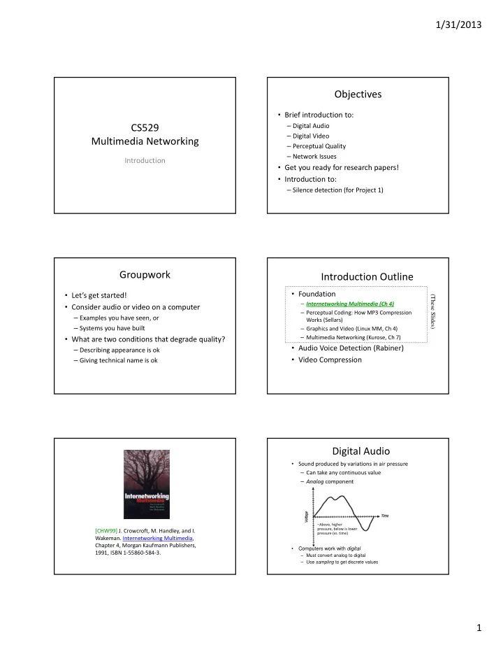
Digital Audio

  • Sound produced by variations in air pressure

– Can take any continuous value – Analog component

  • Computers work with digital

– Must convert analog to digital – Use sampling to get discrete values

–Above, higher pressure, below is lower pressure (vs. time)

slide-2
SLIDE 2

1/31/2013 2

Digital Sampling

  • Sample rate determines number of discrete

values

Digital Sampling

  • Half sample rate

Digital Sampling

  • Quarter sample rate

(How often to sample to reproduce curve?)

Sample Rate

  • Shannon’s Theorem: to accurately reproduce

signal, must sample at twice highest frequency

  • Why not always use high sampling rate?

Sample Rate

  • Shannon’s Theorem: to accurately reproduce

signal, must sample at twice highest frequency

  • Why not always use high sampling rate?

– Requires more storage – Complexity and cost of analog to digital hardware – Human’s can’t always perceive

  • Dog whistle

– Typically want an “adequate” sampling rate

  • “Adequate” depends upon use of reconstructed signal

Sample Size

  • Samples have discrete values
  • How many possible values?
  • Sample Size
  • Say, 256 values from 8 bits
slide-3
SLIDE 3

1/31/2013 3

Sample Size

  • Quantization error from rounding

– Ex: 28.3 rounded to 28

  • Why not always have large sample size?

Sample Size

  • Quantization error from rounding

– Ex: 28.3 rounded to 28

  • Why not always have large sample size?

– Storage increases per sample – Analog to digital hardware becomes more expensive

Groupwork

  • Think of as many uses of computer audio as

you can

  • Which require a high sample rate and large

sample size? Which do not? Why?

Audio

  • Encode/decode devices are called codecs

– Compression is the complicated part

  • For voice compression, can take advantage
  • f speech:

“Smith”

  • Many similarities between adjacent samples
  • Send differences (ADPCM)
  • Use understanding of speech
  • Can ‘predict’ (CELP)

Audio by People

  • Sound by breathing air past vocal cords

– Use mouth and tongue to shape vocal tract

  • Speech made up of phonemes

– Smallest unit of distinguishable sound – Language specific

  • Majority of speech sound from 60‐8000 Hz

– Music up to 20,000 Hz

  • Hearing sensitive to about 20,000 Hz

– Stereo important, especially at high frequency – Lose frequency sensitivity with age

Typical Encoding of Voice

  • Today, telephones carry digitized voice
  • 8000 samples per second

– Adequate for most voice communication

  • 8‐bit sample size
  • For 10 seconds of speech:

– 10 sec x 8000 samp/sec x 8 bits/samp = 640,000 bits or 80 Kbytes – Fit 2 years of raw sound on typical hard disk

  • Ok for voice (but Skype better), but what about

music?

slide-4
SLIDE 4

1/31/2013 4

Typical Encoding of Audio

  • Can only represent 4 KHz frequencies (why?)
  • Human ear can perceive 10‐20 KHz

– Full range used in music

  • CD quality audio:

– sample rate of 44,100 samples/sec – sample size of 16‐bits – 60 min x 60 secs/min x 44100 samp/sec x 2 bytes/samp x 2 channels (stereo) = 635,040,000, about 600 Mbytes (typical CD)

  • Can use compression to reduce

– mp3 (“as it sounds)”, RealAudio – 10x compression rate, same audible quality

Sound File Formats

  • Raw data has samples (interleaved w/stereo)
  • Need way to ‘parse’ raw audio file
  • Typically a header

– Sample rate – Sample size – Number of channels – Coding format – …

  • Examples:

– .au for Sun µ‐law, .wav for IBM/Microsoft – .mp3 for MPEG‐layer 3

Introduction Outline

  • Background

– Internetworking Multimedia (Ch 4) – Perceptual Coding: How MP3 Compression Works (Sellars) – Graphics and Video (Linux MM, Ch 4) – Multimedia Networking (Kurose, Ch 7)

  • Audio Voice Detection (Rabiner)
  • Video Compression

MP3 – Introduction (1 of 2)

  • “MP3” abbreviation of “MPEG 1 audio layer 3”
  • “MPEG” abbrev of “Moving Picture Experts Group”

– 1990, Video at about 1.5 Mbits/sec (1x CD‐ROM) – Audio at about 64‐192 kbits/channel

  • Committee of the International Standards Organization (ISO)

and International Electrotechnical Commission (IEC)

– (Whew! That’s a lot of acronyms (TALOA))

  • MP3 differs in that it does not try to accurately reproduce

PCM (waveform)

  • Instead, uses theory of “perceptual coding”

– PCM attempts to capture a waveform “as it is” – MP3 attempts to capture it “as it sounds”

MP3 – Introduction (2 of 2)

  • Ears and brains imperfect and biased measuring devices,

interpret external phenomena

– Ex: doubling amplitude does not always mean double perceived

  • loudness. Factors (frequency content, presence of any

background noise…) also affect

  • Set of judgments as to what is/not meaningful

– Psychoacoustic model

  • Relies upon “redundancy” and “irrelevancy”

– Ex: frequencies beyond 22 KHz redundant (some audiophiles think it does matter, gives “color”!) – Irrelevancy, discarding part of signal because will not be noticed, was/is new

MP3 ‐ Masking

  • Listener prioritizes sounds ahead of others according to

context (hearing is adaptive)

– Ex: a sudden hand‐clap in a quiet room seems loud. Same hand‐ clap after a gunshot, less loud (time domain) – Ex: guitar may dominate until cymbal, when guitar briefly drowned (frequency domain)

  • Above examples of time‐domain and frequency‐domain

masking, respectively

  • Two sounds occur (near) simultaneously, one may be partially

masked by the other

– Depending relative volumes and frequency content

  • MP3 doesn’t just toss masked sound (would sound odd) but

uses fewer bits for masked sounds

slide-5
SLIDE 5

1/31/2013 5

MP3 – Sub‐Bands (1 of 2)

  • MP3 not method of digital recording

– Instead, removes irrelevant data from existing recording

  • Encoding typically 16‐bit sample size at 32, 44.1 and 48 kHz

sample rate

  • First, short sections of waveform stream filtered

– How, not specified by standard – Typically Fast Fourier Transformation or Discrete Cosine Transformation

  • Method of reformatting signal data into spectral sub‐bands of

differing importance

MP3 – Sub‐Bands (2 of 2)

  • Divide into 32 “sub‐bands” that represent

different parts of frequency spectrum

  • Why frequency sub‐bands? So MP3 can

prioritize bits for each

– Ex:

  • Low‐frequency bass drum, a high‐frequency ride

cymbal, and a vocal in‐between, all at once

  • If bass drum irrelevant, use fewer bits and more for

cymbal or vocals

MP3 – Frames

  • Sub‐band sections are grouped into “frames”
  • Determine where masking in frequency and

time domains will occur

– Which frames can safely be allowed to distort

  • Calculate mask‐to‐noise ratio for each frame

– Use in the final stage of the process: bit allocation

MP3 – Bit Allocation

  • Decides how many bits to use for each frame

– More bits where little masking (low ratio) – Fewer bits where more masking (high ratio)

  • Total number of bits depends upon desired bit rate

– Chosen before encoding by user

  • For quality, a high priority (music) 128 kbps common

– Note, CD is about 1400 kbps, so 10x less

MP3 – Playout and Beyond

  • Save frames (header data for each frame).

Can then play with MP3 decoder.

  • MP3 decoder performs reverse, but simpler

since bit‐allocation decisions are given

– MP3 decoders cheap, fast (ipod!)

  • What does the future hold?

– Lossy compression not needed since bits irrelevant (storage + net)? – Lossy compression so good that all irrelevant bits are banished?

Introduction Outline

  • Background

– Internetworking Multimedia (Ch 4) – Perceptual Coding: How MP3 Compression Works (Sellars) – Graphics and Video (Linux MM, Ch 4) – Multimedia Networking (Kurose, Ch 7)

  • Audio Voice Detection (Rabiner)
  • Video Compression
slide-6
SLIDE 6

1/31/2013 6

[Tr96] J. Tranter. Linux Multimedia Guide, Chapter 4, O'Reilly & Associates, 1996, ISBN: 1565922190

Graphics and Video

“A Picture is Worth a Thousand Words”

  • People are visual by nature
  • Many concepts hard to explain or draw
  • Pictures to the rescue!
  • Sequences of pictures can depict motion

– Video!

Video Images

  • Traditional television is 646x486 (NTSC)
  • HDTV is 1920x1080 (1080p), 1280x720 (720p),

852x480 (480p)

  • Often Internet video smaller

– 352x288 (H.261), 176x144 (QCIF)

  • Monitors higher resolution than traditional TV

(see next slide)

  • Computer video sometimes called “postage

stamp”

– If make full screen, then pixelated (jumbo pixels)

http://en.wikipedia.org/wiki/Display_resolution

Common Display Resolutions

Video Image Components

  • Luminance (Y) and Chrominance: Hue (U) and

Intensity (V) ‐ YUV

– Human eye less sensitive to color than luminance, so those sampled with less resolution (e.g. 4 bits for Y, 2 for U, 2 for V – 4:2:2)

  • YUV has backward compatibility with BW

televisions (only had Luminance)

– Monitors are typically Red Green Blue (RGB) – (Why are primary colors Red Yellow Blue?)

Graphics Basics

  • Display images with graphics hardware
  • Computer graphics (pictures) made up of pixels

– Each pixel corresponds to region of memory – Called video memory or frame buffer

  • Write to video memory

– Traditional CRT monitor displays with raster cannon – LCD monitors align crystals with electrodes

slide-7
SLIDE 7

1/31/2013 7

Monochrome Display

  • Pixels are on (black) or off (white)

– Dithering can make area appear gray

Grayscale Display

  • Bit‐planes: 4 bits per pixel, 24 = 16 gray levels
  • Typically, 8 enough levels for perception (256 human max), but medical

uses (e.g. x‐ray) use 10‐ or 12‐bit since sensors may detect. TIFF, PNG use 16‐bit greyscale.

Color Displays

  • Humans can perceive far more different colors than grayscales

– Cones (color) and Rods (gray) in eyes

  • All colors seen as combo of red, green and blue (additive)
  • Visual maximum needed

– 24 bits/pixel, 224 ~ 16 million colors (true color)

  • Requires 3 bytes per pixel

Sequences of Images – Video (Guidelines)

  • Series of frames with changes appear as

motion

  • Units are frames per second (fps or f/s)

– 24‐30 fps: full‐motion video – 15 fps: full‐motion video approximation – 7 fps: choppy – 3 fps: very choppy – Less than 3 fps: slide show

Video Sizes

  • Raw video bitrate:

color depth * vertical rez * horizontal rez * frame rate e.g. 1080p: 10‐bit (4:4:2) @ 1920 x 1080 @ 29.97fps = ~120 MB per/sec or ~430 GB per/hr Uncompressed video is big!

Video Compression

  • Image compression: about 25 to 1
  • Video compression: about 100 to 1
  • Options: Lossless or Lossy

– (Q: why not always lossless?)

  • Intracoded or Intercoded

– Take advantage of dependencies between frames Motion

(more later)

slide-8
SLIDE 8

1/31/2013 8

Introduction Outline

  • Background

– Internetworking Multimedia (Ch 4) – Perceptual Coding: How MP3 Compression Works (Sellars) – Graphics and Video (Linux MM, Ch 4) – Multimedia Networking (Kurose, Ch 7)

  • Audio Voice Detection (Rabiner)
  • Video Compression

[KR12] J. Kurose and K. Ross. Computer Networking: A Top‐ Down Approach, 6th edition, Pearson, ISBN‐10: 0132856204, 2012.

Section Outline

  • Overview: multimedia on Internet
  • Audio

– Example: Skype

  • Video

– Example: Netflix

  • Protocols

– RTP, SIP

  • Network support for multimedia

Internet Traffic

  • Internet has many text‐based applications

– Email, File transfer, Web browsing

  • Very sensitive to loss

– Example: lose one byte in your blah.exe program and it crashes!

  • Not very sensitive to delay

– 10’s of seconds ok for Web page download – Minutes ok for file transfer – Hours ok for email to delivery

  • Multimedia traffic emerging (especially as

fraction of bandwidth!)

– Video already dominant on some links

Multimedia on the Internet

  • Multimedia not as sensitive to loss

– Words from speech lost still ok – Frames of video missing still ok

  • Multimedia can be very sensitive to delay

– Interactive session needs one‐way delays less than ½ second!

  • New phenomenon is effects of variation in

delay, called delay jitter or just jitter!

– Variation in bandwidth can also be important

Jitter Jitter‐Free

slide-9
SLIDE 9

1/31/2013 9

Multimedia: Audio

  • Analog audio signal

sampled at constant rate phone: 8000 samples/sec CD music: 44,100 samples/sec

  • Each sample quantized

(rounded) e.g., 28=256 possible quantized values each quantized value represented by bits, e.g., 8 bits for 256 values

time audio signal amplitude analog signal quantized value of analog value quantization error sampling rate (N sample/sec)

Multimedia: Audio

  • Example: 8000 samples/sec,

256 quantized values: 64,000 bps

  • Receiver converts bits back

to analog signal: some quality reduction

Example rates

  • CD: 1.411 Mbps
  • MP3: 96, 128, 160 Kbps
  • Internet telephony: 5.3 Kbps

and up

time audio signal amplitude analog signal quantized value of analog value quantization error sampling rate (N sample/sec)

  • Video: sequence of images

displayed at constant rate e.g. 24 images/sec

  • Digital image: array of pixels

each pixel represented by bits

  • Coding: use redundancy

within and between images to decrease # bits used to encode image spatial (within image) temporal (from one image to next)

Multimedia: Video

……………………...…

spatial coding example: instead

  • f sending N values of same

color (all purple), send only two values: color value (purple) and number of repeated values (N)

……………………...… frame i frame i+1

temporal coding example: instead of sending complete frame at i+1, send only differences from frame i

  • CBR (constant bit rate):

video encoding rate fixed

  • VBR (variable bit rate): video

encoding rate changes as amount of spatial, temporal coding changes

  • Examples:

MPEG 1 (CD‐ROM) 1.5 Mb/s MPEG2 (DVD) 3‐6 Mb/s MPEG4 (often used in Internet, < 1 Mb/s)

Some Types of Multimedia Activities over the Internet

  • Streaming, stored audio, video
  • Conversational voice (& video)
  • Streaming live audio, video

Streaming Stored Media

  • Streaming, stored audio, video

– Pre‐recorded – streaming: can begin playout before downloading entire file – stored (at server): can transmit faster than audio/video will be rendered (implies storing/buffering at client)

  • 1‐way communication, unicast
  • Interactivity, includes pause, ff, rewind…
  • Examples: pre‐recorded songs, video‐on‐demand

– e.g. YouTube, Netflix, Hulu

  • Delays of 1 to 10 seconds or so tolerable
  • Need reliable estimate of bandwidth
  • Not very sensitive to jitter
slide-10
SLIDE 10

1/31/2013 10

Conversational Voice/Video

  • Conversational voice/video

– interactive nature of human‐to‐human conversation limits delay tolerance

  • “Captured” from live camera, microphone
  • 2‐way (or more) communication
  • e.g., Skype, Facetime
  • Very sensitive to delay

< 150 ms one‐way delay good < 400 ms ok > 400 ms bad

  • Sensitive to jitter

Streaming Live Media

  • Streaming live audio, video

– streaming: can begin playout before downloading entire file – Not pre‐recorded, so cannot send faster than rendered

  • “Captured” from live camera, microphone
  • May be 1‐way communication, unicast but may be more

– More potential for “flash crowd”

  • Interactivity, includes pause, ff, rewind…
  • Delays of 1 to 10 seconds or so tolerable
  • Need reliable estimate of bandwidth
  • Not very sensitive to jitter
  • Basically, like stored but:

– May be harder to optimize/scale (less time) – May be 2+ recipients (flash crowd)

Hurdles for Multimedia on the Internet

  • IP is best‐effort

– No delivery guarantees – No bitrate guarantees – No timing guarantees

  • So … how do we do it?

– Not as well as we would like – This class is largely about techniques to make it better!

Groupwork: TCP or UDP?

  • Above IP we have UDP and TCP as the de‐facto

transport protocols. Which to use? Streaming, stored audio, video? Conversational voice (& video)? Streaming live audio, video?

TCP or UDP?

  • TCP

+ In order, reliable (no need to control loss) ‐ Congestion control (hard to pick encoding level right)

  • UDP

‐ Unreliable (need to control loss) + Bandwidth control (easier to control sending rate)

An Example: VoIP

(Mini Outline)

  • Specification
  • Removing Jitter
  • Recovering from Loss
slide-11
SLIDE 11

1/31/2013 11

VoIP: Specification

  • 8000 bytes per second, send every 20 msec (why

every 20 msec?)

20 msec * 8000/sec = 160 bytes per packet

  • Header per packet

– Sequence number, time‐stamp, playout delay

  • End‐to‐end delay requirement of 150 – 400 ms

– (So, why might TCP cause problems?)

  • UDP

– Can be delayed different amounts (need to remove jitter) – Can be lost (need to recover from loss)

Client‐side Buffering, Playout

variable fill rate, x(t)

client application buffer, size B

playout rate, e.g., CBR r

buffer fill level, Q(t)

video server client

Client‐side Buffering, Playout

variable fill rate, x(t)

client application buffer, size B

playout rate, e.g., CBR r

buffer fill level, Q(t)

video server client

  • 1. don’t play immediately ‐ initial fill of buffer t0
  • 2. playout begins at tp,
  • 3. buffer fill level varies over time as fill rate x(t) varies

and playout rate r is constant

playout buffering: average fill rate (x), playout rate (r):

  • x < r: buffer eventually empties (causing freezing of video

playout until buffer again fills)

  • x > r: buffer will not empty, provided initial playout delay is large

enough to absorb variability in x(t)

tradeoff: buffer starvation less likely with larger delay, but longer wait until user begins watching

variable fill rate, x(t)

client application buffer, size B

playout rate, e.g., CBR r

buffer fill level, Q(t)

video server

Client‐side Buffering, Playout VoIP: Playout Delay

Playout delay can be fixed or adaptive

Two policies, wait p or wait p’

  • p has less delay, but one missed
  • p’ has no missed, but higher delay
  • Sender generates packets every 20 msec (during

talk spurt)

  • First packet received at time r
  • First playout schedule begins at p
  • Second playout schedule begins at p’

If adaptive, adapt each talkspurt

VoIP: Loss

1 2 3 4

Encode

1

Transmit

4 1 ??? 4

Decode

??? Q: What to do about missing packets?

slide-12
SLIDE 12

1/31/2013 12

VoIP: Recovering from Loss

1 2 3 1 1 1 2 3 4

Encode

3 4

Decode

1

Transmit

4 3

supernode

  • verlay

network

Voice‐over‐IP: Skype

  • Proprietary application‐

layer protocol (inferred via reverse engineering)

– encrypted msgs

  • P2P components:

Skype clients (SC)

  • clients (SC): Skype peers

connect directly to each

  • ther for

VoIP call

  • super nodes (SN): Skype

peers with special functions

  • verlay network: among SNs to

locate SCs

  • login server

Skype login server

supernode (SN)

P2P Voice‐over‐IP: Skype

Skype client operation:

  • 1. joins Skype network by

contacting SN (IP address cached) using TCP

  • 2. logs-in (usename, password) to

centralized Skype login server

  • 3. obtains IP address for callee

from SN, SN overlay

  • r client buddy list
  • 4. initiate call directly to callee

Skype login server

Q: when might this not work?

  • Problem: both Alice, Bob

behind “NATs”

– NAT prevents outside peer from initiating connection to insider peer – inside peer can initiate connection to outside

  • Relay solution: Alice, Bob

maintain open connection to their SNs

  • Alice signals her SN to connect to

Bob

  • Alice’s SN connects to Bob’s SN
  • Bob’s SN connects to Bob over
  • pen connection Bob initially

initiated to his SN

Skype: Peers as Relays Projects

  • Project 1:

– Read and Playback from audio device – Detect Speech and Silence – Evaluate (1a)

  • Project 2:

– Build a VoIP application – Evaluate (2b)

  • Project 3:

– Pick your own (video conf, thin game, repair …)

Section Outline

  • Overview: multimedia on Internet

(done)

  • Audio

(done)

– Example: Skype (done)

  • Video

(next)

– Example: Netflix

  • Protocols

– RTP, SIP

  • Network support for multimedia
slide-13
SLIDE 13

1/31/2013 13

Streaming Stored Video

  • 1. video

recorded (e.g., 30 f/s)

  • 2. video

sent streaming: at this time, client playing out early part of video, while server still sending later part of video network delay (fixed in this example) time

  • 3. video received,

played out at client (30 f/s)

Streaming Stored Video: Challenges

  • Continuous playout constraint: once client

playout begins, playback must match original timing

  • … but network delays are variable (jitter), so will

need client-side buffer to match playout requirements

  • Other challenges:
  • client interactivity: pause, fast-forward, rewind, jump

through video

  • video packets may be lost, retransmitted

constant bit rate video transmission time variable network delay client video reception constant bit rate video playout at client client playout delay

buffered video

  • client‐side buffering: compensates for delay

jitter and bitrate jitter

Streaming Stored Video: Revisted Streaming Multimedia: UDP

  • Server sends at rate appropriate for client

– Often: send rate = encoding rate = constant rate – Transmission rate can be oblivious to congestion levels!

  • Short playout delay (2‐5 seconds) to remove

bandwidth (and delay) jitter

  • Error recovery: application‐level, time

permitting

  • RTP [RFC 2326]: multimedia payload types (later)
  • UDP often not allowed through firewalls

Streaming Multimedia: HTTP

  • Basis for many: Apple, Microsoft Silverlight, Adobe, Netfilx
  • Multimedia file retrieved via HTTP GET
  • Send at maximum possible rate under TCP
  • Fill rate fluctuates due to TCP congestion control,

retransmissions (in‐order delivery)

  • Larger playout delay to smooth out TCP delivery rate
  • HTTP/TCP passes more easily through firewalls

variable rate, x(t) TCP send buffer video file TCP receive buffer application playout buffer

server client

Streaming Multimedia: DASH

  • DASH: Dynamic, Adaptive Streaming over HTTP

– Now a standard, basis for Netflix streaming

  • Server:

– divides video file into multiple chunks – each chunk stored, encoded at different rates – manifest file: provides URLs for different chunks

  • Client:

– periodically measures server‐to‐client bandwidth – consulting manifest, requests one chunk at a time

  • chooses maximum coding rate sustainable given current

bandwidth

  • can choose different coding rates at different points in time

(depending on available bandwidth at time)

slide-14
SLIDE 14

1/31/2013 14

Streaming Multimedia: DASH

  • “intelligence” at client: client determines

– when to request chunk (so that buffer starvation, or overflow does not occur) – what encoding rate to request (higher quality when more bandwidth available) – where to request chunk (can request from URL server that is “close” to client or has high available bandwidth)

Content Distribution Networks

  • challenge: how to stream content (selected

from millions of videos) to hundreds of thousands of simultaneous users?

  • option 1: single, large “mega‐server”

– single point of failure – point of network congestion – long path to distant clients – multiple copies of video sent over outgoing link

….quite simply: this solution doesn’t scale

Content Distribution Networks

  • challenge: how to stream content (selected

from millions of videos) to hundreds of thousands of simultaneous users?

  • option 2: store/serve multiple copies of videos at

multiple geographically distributed sites (content distribution network, or CDN)

– enter deep: push CDN servers deep into many access networks

  • close to users
  • used by Akamai, 1700 locations

– bring home: smaller number (10’s) of larger clusters in near (but not within) access networks

  • used by Limelight

CDN: “Simple” Content Access Scenario

Bob (client) requests video http://netcinema.com/6Y7B23V

  • video stored in CDN at http://KingCDN.com/NetC6y&B23V

netcinema.com KingCDN.com

1

  • 1. Bob gets URL for for video

http://netcinema.com/6Y7B23V from netcinema.com Web page 2

  • 2. resolve http://netcinema.com/6Y7B23V

via Bob’s local DNS

netcinema’s authorative DNS

3 4 4&5. Resolve http://KingCDN.com/NetC6y&B23 via KingCDN’s authoritative DNS, which returns IP address of KingCDN server with video 5

  • 6. request video from

KINGCDN server, streamed via HTTP

KingCDN authoritative DNS

  • 3. netcinema’s DNS returns URL

http://KingCDN.com/NetC6y&B23V

CDN Cluster Selection Strategy

  • challenge: how does CDN DNS select “good”

CDN node to stream to client

– pick CDN node geographically closest to client – pick CDN node with shortest delay (or min # hops) to client (CDN nodes periodically ping access ISPs, reporting results to CDN DNS) – IP anycast – same addresses routed to one of many locations (routers pick, often shortest hop)

  • alternative: let client decide ‐ give client a list
  • f several CDN servers

– client pings servers, picks “best” – Netflix approach?

Case Study: Netflix

slide-15
SLIDE 15

1/31/2013 15

Netflix Overview

  • 20+ million subscribers in

2011 (15% of US households)

  • 20% downstream US traffic

at peak hours

  • Bitrates up to 4.8 Mb/s
  • Known for

“recommendations”

  • Many Netflix‐ready devices

(next slide)

Netflix Partner Products Netflix Network Approach

Client‐centric

  • Client has best view of

network conditions

  • No session state in network

– Better scalability

  • But, must rely upon client

for operational metrics

– Only client knows what happened, really

CDN

  • Own little infrastructure, use 3rd

parties

– Own registration, payment servers

  • Amazon cloud services:

– Cloud hosts Netflix web pages for user browsing – Netflix uploads studio master to Amazon cloud

– Create multiple version of movie (different

encodings) in cloud

– Upload versions from cloud to CDNs

  • Three 3rd party CDNs host/stream

Netflix content: Akamai, Limelight, Level‐3

Netflix – Initiate Request

1

  • 1. Bob manages

Netflix account Netflix registration, accounting servers Amazon cloud Akamai CDN Limelight CDN Level-3 CDN 2

  • 2. Bob browses

Netflix video 3

  • 3. Manifest file

returned for requested video

  • 4. DASH

streaming upload copies of multiple versions of video to CDNs

Netflix Importance of Client Metrics

  • Metrics are essential

– Detecting and debugging failures – Managing performance – Experimentation (new interfaces, features)

  • Absence of server‐side metrics places onus on

client

  • What is needed?

– Reports of what user did (or didn’t) see

  • Which part of which stream when

– Reports of what happened in network

  • Requests sent, responses received, timing, throughput

Netflix Quality

  • Reliable transport (HTTP is over TCP)
  • Quality characterized by

– Video quality (how it looks)

  • At startup, average and variability (different layers)

– Startup delay

  • Time form use action to first frame displayed

– Rebuffer rate

  • Rebuffers per viewing hour, duration of rebuffer pauses
slide-16
SLIDE 16

1/31/2013 16

Netflix Performance of Top US Networks

Netflix Streaming Bitrates

(one device type)

  • Cyclic session hours (Q: why?)
  • Average bitrate stays relatively flat (but not totally)

Netflix Rebuffer Rates

  • Rebuffers at peaks for sessions (usually)
  • Worst is about 1‐2 per hour
  • CDN performance is better

Netflix Adaptation Problem

  • At client, pick sequence and timing of requests in
  • rder to:

– minimize probability of rebuffering – maximize visual quality

Netflix Adaptation Approach

  • Example:

– Model future bandwidth: constant? avg over last 10s? – Analyze choices: construct “plan” for each choice, know visual quality, estimate rebuffering

NetFlix Future Work Needs

  • Good models of future bandwidth (based on

history)

– Short term history – Long term history (across multiple sessions)

  • Tractable representations of future choices

– Including scalability, multiple streams

  • Quality goals with “right” mix of visual quality

and performance (rebuffering)

  • Convolution of future bandwidth models with

possible plans

– Efficiently, maximizing quality goals

slide-17
SLIDE 17

1/31/2013 17

Section Outline

  • Overview: multimedia on Internet

(done)

  • Audio

(done)

– Example: Skype (done)

  • Video

(done)

– Example: Netflix (done)

  • Protocols

(next)

– RTP, SIP

  • Network support for multimedia

Real‐Time Protocol (RTP) [RFC 3550]

  • RTP specifies packet

structure for packets carrying audio, video data

  • RTP packet provides

– payload type identification – packet sequence number – time stamp

  • RTP runs in end systems,

not routers

  • RTP packets encapsulated

in UDP segments

  • Interoperability potential

– e.g. if two VoIP applications run RTP, they may be able to work together

RTP Runs on Top of UDP

  • RTP libraries provide transport‐layer interface

that extends UDP:

– Port numbers, IP addresses – Payload type identification – Packet sequence numbers – Time stamps

RTP Example

Example: sending 64 kb/s PCM‐encoded voice over RTP

  • application collects

encoded data in chunks, e.g., every 20 msec = 160 bytes in chunk

  • audio chunk + RTP

header form RTP packet encapsulated in UDP segment

  • RTP header indicates

type of audio encoding in each packet

– sender can change encoding during conference

  • RTP header also

contains sequence numbers, timestamps

RTP and Quality of Service (QoS)

  • RTP does not provide any mechanism to

ensure timely data delivery or other QoS guarantees

  • RTP encapsulation only seen at end systems

(not by intermediate routers)

– routers provide best‐effort service, making no special effort to ensure that RTP packets arrive at destination in timely matter

Real‐Time Control Protocol (RTCP)

  • Works in conjunction with

RTP

  • Each participant in RTP

session periodically sends RTCP control packets to all other participants

  • Each RTCP packet

contains sender and/or receiver reports

– report statistics useful to application: # packets sent, # packets lost, interarrival jitter

  • Feedback used to control

performance

– sender may modify its transmissions based on feedback

RTCP RTP RTCP RTCP

sender receivers

slide-18
SLIDE 18

1/31/2013 18

SIP: Session Initiation Protocol [RFC 3261]

Long‐term vision:

  • All telephone calls, video

conference calls take place over Internet

  • People identified by

names or e‐mail addresses, rather than by phone numbers

  • Can reach callee (if callee

so desires), no matter where callee roams, no matter what IP device callee is currently using

  • SIP comes from IETF:

borrows much of its concepts from HTTP

– SIP has “Web flavor” – Alternative approaches (e.g. H.323) have “telephony flavor”

  • SIP uses KISS principle:

Keep It Simple Stupid

SIP Services

  • SIP provides

mechanisms for call setup:

– for caller to let callee know s/he wants to establish a call – so caller, callee can agree on media type, encoding – to end call

  • Determine current IP

address of callee:

– maps mnemonic identifier to current IP address

  • Call management:

– add new media streams during call – change encoding during call – invite others – transfer, hold calls

Example: Setting Up Call to Known IP Address

  • Alice’s SIP invite message

indicates her port number, IP address, encoding she prefers to receive (PCM µlaw)

  • Bob’s 200 OK message

indicates his port number, IP address, preferred encoding (GSM)

  • SIP messages can be sent
  • ver TCP or UDP; here

sent over RTP/UDP

  • Default SIP port is 5060

time time Bob's terminal rings Alice 167.180.112.24 Bob 193.64.210.89 port 5060 port 38060 µ Law audio GSM port 48753 INVITE bob@193.64.210.89 c=IN IP4 167.180.112.24 m=audio 38060 RTP/AVP 0 port 5060 2 O K c = I N I P 4 1 9 3 . 6 4 . 2 1 . 8 9 m = a u d i

  • 4

8 7 5 3 R T P / A V P 3 ACK port 5060

Setting Up a Call (more)

  • Codec negotiation:

– suppose Bob doesn't have PCM µlaw encoder – Bob will instead reply with 606 Not Acceptable reply, listing his encoders. Alice can then send new INVITE message, advertising different encoder

  • Rejecting call

– Bob can reject with replies “busy,” “gone,” “payment required,” “forbidden”

  • Media can be sent
  • ver RTP or some
  • ther protocol

SIP Name Translation, User location

  • Caller wants to call

callee, but only has callee’s name or e‐mail address.

  • Need to get IP address of

callee’s current host:

– user moves around – DHCP protocol – user has different IP devices (PC, smartphone, car device)

  • Result can be based on:

– time of day (work, home) – caller (don’t want boss to call you at home) – status of callee (calls sent to voicemail when callee is already talking to someone)

SIP Registrar

REGISTER sip:domain.com SIP/2.0 Via: SIP/2.0/UDP 193.64.210.89 From: sip:bob@domain.com To: sip:bob@other-domain.com Expires: 3600

  • One function of SIP server: registrar
  • When Bob starts SIP client, client sends SIP

REGISTER message to Bob’s registrar server register message:

slide-19
SLIDE 19

1/31/2013 19

SIP Proxy

  • Another function of SIP server: proxy
  • Alice sends invite message to her proxy server

– contains address sip:bob@domain.com – proxy responsible for routing SIP messages to callee, possibly through multiple proxies

  • Bob sends response back through same set of SIP

proxies

  • Proxy returns Bob’s SIP response message to Alice

– contains Bob’s IP address

  • SIP proxy analogous to local DNS server plus TCP

setup

SIP Example: jim@umass.edu Calls keith@poly.edu

1

  • 1. Jim sends INVITE

message to UMass SIP proxy.

  • 2. UMass proxy forwards request

to Poly registrar server 2

  • 3. Poly server returns redirect response,

indicating that it should try keith@eurecom.fr 3

  • 5. eurecom

registrar forwards INVITE to 197.87.54.21, which is running keith’s SIP client 5 4

  • 4. Umass proxy forwards request

to Eurecom registrar server 8 6 7 6-8. SIP response returned to Jim 9

  • 9. Data flows between clients

UMass SIP proxy Poly SIP registrar Eurecom SIP registrar 197.87.54.21 128.119.40.186

Section Outline

  • Overview: multimedia on Internet

(done)

  • Audio

(done)

– Example: Skype (done)

  • Video

(done)

– Example: Netflix (done)

  • Protocols

(done)

– RTP, SIP (done)

  • Network support for multimedia

(next)

Network Support for Multimedia

  • Most of Internet is “best effort” and is focus of this class
  • But there is some differentiated services
  • And issues are useful for all

Capacity Planning in Best Effort Networks

  • Approach: deploy enough link capacity so that

congestion doesn’t occur, multimedia traffic flows without delay or loss

– low complexity of network mechanisms (use current “best effort” network) – high bandwidth costs

  • Challenges:

– capacity planning: how much bandwidth is “enough?” – estimating network traffic demand: needed to determine how much bandwidth is “enough” (for that much traffic)

Providing Multiple Classes of Service

  • Thus far: making the best of best effort service

– “one‐size fits all” service model

  • Alternative: multiple classes of service

– partition traffic into classes – network treats different classes of traffic differently (analogy: VIP service versus regular service)

0111

  • Granularity:

differential service among multiple classes, not among individual connections

slide-20
SLIDE 20

1/31/2013 20

Scenario: Mixed HTTP and VoIP

  • Example: 1 Mbps VoIP & HTTP share 1.5 Mb/s link.

– HTTP bursts can congest router, cause VoIP loss – Want to give priority to VoIP over HTTP Packet marking needed for router to distinguish between different classes; and new router policy to treat packets accordingly

Principle 1

R1 R2

1.5 Mbps link R1 output interface queue

Principles for QOS Guarantees

  • What if applications misbehave (VoIP sends higher

than declared rate)?

– policing: force source adherence to bandwidth allocations

  • Marking, policing at network edge

Provide protection (isolation) for one class from others

Principle 2

R1 R2

1.5 Mbps link 1 Mbps phone

packet marking and policing

  • Allocating fixed (non‐sharable) bandwidth to

flow? Inefficient use of bandwidth if flows doesn’t use its allocation

While providing isolation, it is desirable to use resources as efficiently as possible Principle 3

R1 R2

1.5 Mbps link 1 Mbps phone 1 Mbps logical link 0.5 Mbps logical link

Principles for QOS Guarantees Scheduling and Policing Mechanisms

  • Scheduling: choose next packet to send on link
  • FIFO (first in first out) scheduling: send in order of

arrival to queue

– real‐world example? – discard policy: if packet arrives to full queue: who to discard?

  • tail drop: drop arriving packet
  • priority: drop/remove on priority basis
  • random: drop/remove randomly

queue (waiting area) packet arrivals packet departures link (server)

Q: other policies?

Scheduling Policies: Priority

Priority scheduling: send highest priority queued packet

  • Multiple classes,

with different priorities

– class may depend

  • n marking or other

header info, e.g. IP source/dest, port numbers, etc. – real world example?

high priority queue (waiting area) low priority queue (waiting area) arrivals classify departures link (server)

1 3 2 4 5 5 5 2 2 1 1 3 3 4 4

arrivals departures packet in service

Scheduling Policies: Still More

Round Robin (RR) scheduling:

  • multiple classes
  • cyclically scan class queues, sending one complete packet

from each class (if available)

  • real world example?

1 2 3 4 5 5 5 2 3 1 1 3 3 4 4

arrivals departures packet in service

slide-21
SLIDE 21

1/31/2013 21

Weighted Fair Queuing (WFQ):

  • Generalized Round Robin
  • Each class gets weighted amount of service in

each cycle

  • real‐world example?

Scheduling Policies: Still More Policing Mechanisms

Goal: limit traffic to not exceed declared parameters Three commonly‐used criteria:

  • (long term) average rate: how many packets can be

sent per unit time (in long run)

– crucial question: what is the interval length: 100 packets per sec or 6000 packets per min have same average!

  • peak rate: e.g., 600 pkts per min (ppm) avg.; 1500 ppm

peak rate

  • (max) burst size: max number of pkts sent

consecutively (with no intervening idle)

Policing Mechanisms: Implementation

token bucket: limit input to specified burst size (b) and average rate (r)

  • Bucket can hold b tokens
  • Tokens generated at rate r token/sec unless bucket full
  • Over interval of length t: number of packets admitted

less than or equal to (r t + b)

Policing and QoS Guarantees

  • Token bucket, WFQ combine to provide

guaranteed upper bound on delay, i.e., QoS guarantee!

WFQ

token rate, r bucket size, b

per-flow rate, R D = b/R max

arriving traffic arriving traffic

Differentiated Services (DiffServ)

  • Want “qualitative” service classes

– “behaves like a wire” – Relative service distinction: Platinum, Gold, Silver

  • Scalability: simple functions in network core,

relatively complex functions at edge routers (or hosts)

– signaling, maintaining per‐flow router state difficult with large number of flows

  • Don’t define service classes, provide functional

components to build service classes

Edge router:

  • per-flow traffic management
  • marks packets as in-profile and
  • ut-profile

Core router:

  • per class traffic management
  • buffering and scheduling based
  • n marking at edge
  • preference given to in-profile

packets over out-of-profile packets

DiffServ Architecture

r b

marking scheduling

. . .

slide-22
SLIDE 22

1/31/2013 22

Per‐connection QoS Guarantees

  • basic fact: cannot support traffic demands

beyond link capacity

call admission: flow declares its needs, network may block call (e.g., busy signal) if it cannot meet needs Principle 4

R1 R2

1.5 Mbps link 1 Mbps phone 1 Mbps phone

QoS Guarantee Scenario

  • Resource reservation

– call setup, signaling (RSVP) – traffic, QoS declaration – per‐element admission control QoS-sensitive scheduling (e.g., WFQ)

request/ reply

Introduction Outline

  • Foundation

(done)

– Internetworking Multimedia (Ch 4) (done) – Perceptual Coding: MP3 Compression (done) – Graphics and Video (Linux MM, Ch 4) (done) – Multimedia Networking (Kurose, Ch 7) (done)

  • Audio Voice Detection (Rabiner)

(done)

  • Video Compression

(next)

– (Next slide deck)