Notes for 848 lecture 4: A ML basis for compatibility and parsimony - - PDF document

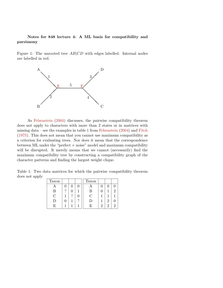
Notes for 848 lecture 4: A ML basis for compatibility and parsimony Figure 1: The unrooted tree AB|CD with edges labelled. Internal nodes are labelled in red. A B D C 1 2 3 4 5

❅ ❅ ❅ ❅ ❅

• E

F

• ❅

❅ ❅ ❅ ❅

As Felsenstein (2004) discusses, the pairwise compatibility theorem does not apply to characters with more than 2 states or in matrices with missing data – see the examples in table 1 from Felsenstein (2004) and Fitch (1975). This does not mean that you cannot use maximum compatibility as a criterion for evaluating trees. Nor does it mean that the correspondence between ML under the “perfect + noise” model and maximum compatibility will be disrupted. It merely means that we cannot (necessarily) find the maximum compatibility tree by constructing a compatibility graph of the character patterns and finding the largest weight clique. Table 1: Two data matrices for which the pairwise compatibility theorem does not apply Taxon A B ? 1 C 1 ? D 1 ? E 1 1 1 Taxon A B 1 2 C 1 1 1 D 1 2 E 2 2 2

Is our model reasonable?

We have just derived a model that justifies the use of selection of trees using the maximum compatibility. Is the model biologically plausible? No, and it is not even close. First of all, the perfect data portion

• f the model assumed that (for characters within this class) homoplasy is

impossible – that seems too drastic for the types of characters that we usually

• study. Second the “noise” category assumes that the imperfect characters

contain no phylogenetic information – that also seems extreme. This could happen if the noisy characters were evolving at an extremely high (essentially infinite) rate but this is not too plausible (Felsenstein, 1981, provides a derivation of the connection between maximum compatibility and a mixture

• f low rate and high rate characters like the one presented above)

We will discuss model selection later in the class. Very briefly, it is done be comparing the likelihood between alternate models and assessing whether or not there is “significantly” better fit base on the likelihood ratio and some description of how complex the two models are. We don’t always need another model in hand to ask if a model is a good fit for the data. For example one implication under our perfect+noise model is that we would see no phylogenetic signal in the characters that do not fit the tree perfectly. In fact if we use some summary statistic such as the minimum number of changes required to explain a character (the parsimony score), then we find that real data sets show much more phylogenetic signal among characters that have some homoplasy than we would expect if all the homoplasy were being generated by a +noise type of model (PTP results from the Graybeal Cannatella dataset).

More realistic models that produce character con- flict

Rather than assume that incorrect homology statements are an “all-or- nothing” situation (perfect coding for a column or no information at all), it seems reasonable to consider a model in which multiple changes can occur across the tree. Because the state space is not infinite this can result in

homplasy – convergence, parallelism, reversion. In all cases we could imag- ine the homplasy to be “biological” (actual acquisition of the same state in every possible detail), or the result of mis-coding similar states as the same discrete state code. While these two forms of homoplasy sound very different, they really blend into each other. And it may not be crucial to distinguish between them when modeling morphological data.

No filtering of data

Let’s develop the next few sections without conditioning on the fact that our data is variable (the results won’t change substantively for the points that we’d like to make, but it will make the formulation more straightforward).

More realistic models that produce character con- flict

For the time being, we will continue to consider models for which there is an equal probability of change across each branch of the tree. But in this case we will allow more than one change across the tree. For the four taxon tree shown in figure 1, there are 5 branches, so there could be from zero to five transitions on the tree (if we consider only the endpoints of an edge and assume that we cannot detect multiple state changes across a single branch). On this per-branch basis there are 25 = 32 possible character histories possible. However, if we polarize the characters with 0 as the state in A, then we see recall that there are only 8 possible

• patterns. The difference in numbers is accounted for by the fact the there

are two internal nodes (E and F in figure 1) that are unsampled. Each of the internal nodes can have any of the states so there are 22 = 4 different ways to obtain each pattern. Let’s refer to the probability of a change across a single edge (any edge in the tree) as p: If there are only two states, then there are only two possible outcomes for transitions across an edge: no change, or change to the other state. By the law of total probability, the probability of no change must be 1 − p.

By assuming that a change (or lack of change) on one branch of the tree is independent of the probability of change on another branch, we can calculate probability of a character history as the product of the probabilities

• f the transitions. Table 2 shows the pattern probabilities under our equal-

branch length model. They are considerably more complex than those that we encountered under our perfect+noise model because we have to consider all possible character state transformations. The table looks intimidating, but we can detect some reassuring fea- tures:

• All of the terms in the probability summation have a total power of

5 when we consider the exponents on p and on (1 − p). This reflects that fact that there are 5 branches and an event (change in state or no change in state) occurs across each branch.

• All four of the “autapomorphy” patterns have the same probability.
• The Pr(0110) = Pr(0101) on the A+B tree, but Pr(0011) = Pr(0101).

Thus the character with the synapomorphy on the tree seems to have a different fit than the two characters that are incompatible with the tree.

• symmetry arguments imply that if we consider another tree under

this model, then the only patter frequencies that will change are the probabilities of the 0110, 0101, and 0011 patterns (and the frequencies will be simply relabeling of the those shown in table 2 How can we get a feel for the different probabilities? We can plot them as a function of p. See figure 2. Note that when p is very small we expect to see mainly constant characters. This makes sense. The proba- bilities converge as p → 0.5; this also makes sense, when p = 0.5 there is no phylogenetic information (knowing the starting state of an edge tells you nothing about the state at the end of the edge) and we are back to the noise model that implies that all patterns are equiprobable. We can also think about what happens when p → 0. As this happens, the terms that have higher powers of p start to become negligible. When p is a tiny, positive number: p0 ≫ p1 ≫ p2 ≫ p3 ≫ p4 ≫ p5 If we drop the higher order terms we get the pattern frequencies shown in

Table 2: The probability of data patterns on the tree shown in figure 1. The four middle columns are the probability of the pattern with specific states for the internal nodes (E and F in the figure). The last column (the pattern likelihood) is simply the sum of these four history probabilities. Internal state (E,F) leaf pattern (0,0) (0,1) (1,0) (1,1) Pr(pattern|TAB) 0000 (1 − p)5 (1 − p)2p3 (1 − p)2p3 (1 − p)p4 (1 − p)5 + 2(1 − p)2p3 + (1 − p)p4 0001 (1 − p)4p (1 − p)3p2 (1 − p)p4 (1 − p)2p3 (1 − p)4p + (1 − p)3p2 + (1 − p)2p3 + (1 − p)p4 0010 (1 − p)4p (1 − p)3p2 (1 − p)p4 (1 − p)2p3 (1 − p)4p + (1 − p)3p2 + (1 − p)2p3 + (1 − p)p4 0011 (1 − p)3p2 (1 − p)4p p5 (1 − p)3p2 (1 − p)4p + 2(1 − p)3p2 + p5 0100 (1 − p)4p (1 − p)p4 (1 − p)3p2 (1 − p)2p3 (1 − p)4p + (1 − p)3p2 + (1 − p)2p3 + (1 − p)p4 0101 (1 − p)3p2 (1 − p)2p3 (1 − p)2p3 (1 − p)3p2 2(1 − p)3p2 + 2(1 − p)2p3 0110 (1 − p)3p2 (1 − p)2p3 (1 − p)2p3 (1 − p)3p2 2(1 − p)3p2 + 2(1 − p)2p3 0111 (1 − p)2p3 (1 − p)3p2 (1 − p)p4 (1 − p)4p (1 − p)4p + (1 − p)3p2 + (1 − p)2p3 + (1 − p)p4 Figure 2: Pattern frequencies as a function of the per-branch probability of change.

0.0 0.1 0.2 0.2 0.3 0.4 0.5 0.4 0.6 0.8 1.0

0000 0011 0001 0101

table 3. Based on this simplification we can see that as p becomes very small: Pr(constant) ≫ Pr(autapo) = Pr(synapo) ≫ Pr(homoplasy) Note that the terms that dominate the likelihood in this case are those terms which have the fewest number of changes of state. In fact the exponent of p in the approximate likelihood is equal to the minimal number of steps required to explain the character on that tree. As you would probably guess, finding the ML tree under this model is very similar to minimizing the total number

• f steps on the tree.

Table 3: An approximation of the probability of data patterns on the tree shown in figure 1 made by dropping terms that do not have the minimal exponent for p. Terms that were dropped are shown in red; Table 2 shows the full (non approximate) probabilities. The final column provides an even rougher approximation by setting 1 − p ≈ 1. Internal state (E,F) di (0,0) (0,1) (1,0) (1,1) limp→0 Pr(di|TAB) ≈ limp→0 Pr(di|TAB) 0000 (1 − p)5 (1 − p)2p3 (1 − p)2p3 (1 − p)p4 (1 − p)5 1 0001 (1 − p)4p (1 − p)3p2 (1 − p)p4 (1 − p)2p3 (1 − p)4p p 0010 (1 − p)4p (1 − p)3p2 (1 − p)p4 (1 − p)2p3 (1 − p)4p p 0011 (1 − p)3p2 (1 − p)4p p5 (1 − p)3p2 (1 − p)4p p 0100 (1 − p)4p (1 − p)p4 (1 − p)3p2 (1 − p)2p3 (1 − p)4p p 0101 (1 − p)3p2 (1 − p)2p3 (1 − p)2p3 (1 − p)3p2 2(1 − p)3p2 2p2 0110 (1 − p)3p2 (1 − p)2p3 (1 − p)2p3 (1 − p)3p2 2(1 − p)3p2 2p2 0111 (1 − p)2p3 (1 − p)3p2 (1 − p)p4 (1 − p)4p (1 − p)4p p

Is the equal branch length model a parsimony model?

As we just discussed, when the probability of change is low, the likelihood under our equal-branch length model is dominated by the number of changes. Because we take the product over all patterns to get a dataset’s likelihood, the likelihood will be dominated by the sum of the number of steps required

to explain the data. This seems to lead us to the conclusion that the par- simony criterion: prefer the tree with the fewest number of steps needed to explain the data is an ML estimator under the equal branch length model. This is not true – but for almost all datasets that you would encounter it is quite likely that the most parsimonious tree will maximize the equal branch length model. A simple counterexample showing that the MP and ML-equal-branch lengths are not the same is given in table 4. In this example there is a synapormorphy supporting each tree, and there are two partially scored characters that indicate a difference between A and C and A and D,

• respectively. The first three characters (taken together) do not support any

tree, but the divergent character states from A to C and to D are easier to explain on the AB tree. Note that if we ignore higher order terms (when p close to 0) the likelihood for the last two characters are: Pr(0?1?|TAB) = Pr(0??1|TAB) ≈ 3p (1) Pr(0?1?|TAC) ≈ 2p (2) Pr(0??1|TAC) ≈ 3p (3) Pr(0?1?|TAD) ≈ 3p (4) Pr(0??1|TAD) ≈ 2p (5) This reflects that fact that there are three branches that could display a change on the AB tree on characters that resemble a character shown in figure 3, but only two branches that provide an opportunity for a change for characters 4 The example in table 4 is simple but artificial. It is tempting to think that, perhaps if we are given enough data then parsimony and ML under the equal branch length model will always converge to the same tree. In fact this is not the case (for general values of p). Kim (1996) shows an example

• f an (admittedly unrealistic) tree shape which has equal branch lengths.

Given an unlimited amount of data parsimony recovers one tree (not the correct tree), but ML methods would recover the true tree.

Table 4: A data set for which ML under the equal-branch model prefers tree A+B, but MP does not prefer a tree. In the table, psyn = (1 − p)4p + 2(1−p)3p2+p5, this is the probability of a synapomorphy that is compatible with the tree. The probability of a incompatible character pattern is pinc = 2(1 − p)3p2 + 2(1 − p)2p3 Characters Taxon A B 1 1 ? ? C 1 1 1 ? D 1 1 ? 1 Tree Prob. TAB psyn pinc pinc 3p(1 − p)2 + p3 3p(1 − p)2 + p3 TAC pinc psyn pinc 2p(1 − p) 3p(1 − p)2 + p3 TAD pinc pinc psyn 3p(1 − p)2 + p3 2p(1 − p) Goldman (1990) pointed out that if you use ML to infer not just the tree, but also the set of ancestral character states, then you will always prefer the same tree as parsimony. This amounts to using just one possible set of internal nodes assignments for each character. If the parsimony length of character i is si(T), then the reconstruc- tion with the highest likelihood will be one of the reconstructions with the probability of psi(T)(1 − p)2N−3−si(T). The overall likelihood will be: S(T) =

M

• i=1

si(T) (6) Pr(X|T) = pS(T)(1 − p)(2NM−3M−S(T)) (7) Because 0 < p < (1 − p) < 1 and N and M are constant across all trees, minimizing S(T) will maximize the likelihood.

References

Felsenstein, J. (1981). A likelihood approach to character weighting and what it tells us about parsimony and compatibility. Biological Journal of

Figure 3: A character that could be explained by one change on one of 3 branches. ? ? 1

❅ ❅ ❅ ❅ ❅

• ❅

❅ ❅ ❅ ❅

Figure 4: A character that could be explained by one change on one of 2 branches. 1 ? ?

❅ ❅ ❅ ❅ ❅

• ❅

❅ ❅ ❅ ❅

the Linnean Society, 16:183–196. Felsenstein, J. (2004). Inferring Phylogenies. Sinauer Associates, Inc, Sun- derland, Massachusetts, 1 edition. Fitch, W. M. (1975). toward finding the tree of maximum parsimony. In Es- tabrook, G. F., editor, Proceedings of the Eighth International Conference

• n Numerical Taxonomy, San Francisco, CA. W. H. Freeman.

Goldman, N. (1990). Maximum likelihood inference of phylogenetic trees, with special reference to a poisson process model of DNA substitution and to parsimony analyses. Systematic Zoology, 39(4):345–361. Kim, J. (1996). General inconsistency conditions for maximum parsimony: Effects of branch lengths and increasing number of taxa. Systematic Bi-

• logy, 45:363–374.