normative modelling of the visual system predicting
play

Normative Modelling of the Visual System Predicting Retinal Ganglion - PowerPoint PPT Presentation

Normative Modelling of the Visual System Predicting Retinal Ganglion Cell Receptive Fields Book: HHH [Hyv arinen et al., 2009] (free online) Natural Image Statistics: A Probabilistic Approach to Early Computational Vision , Springer 2009,


  1. Normative Modelling of the Visual System Predicting Retinal Ganglion Cell Receptive Fields Book: HHH [Hyv¨ arinen et al., 2009] (free online) Natural Image Statistics: A Probabilistic Approach to Early Computational Vision , Springer 2009, chapter 1 based on material by Chris Williams & Mark van Rossum Normative vs Descriptive Theories: how should the system behave? Of course, this makes most sense if evolution has optimized the Neural Information Processing School of Informatics, University of Edinburgh natural system. Effect of constraints “Statistical-ecological” approach February 2018 Chapter 10 of Dayan and Abbott (2001) is also useful. 1 / 24 2 / 24 
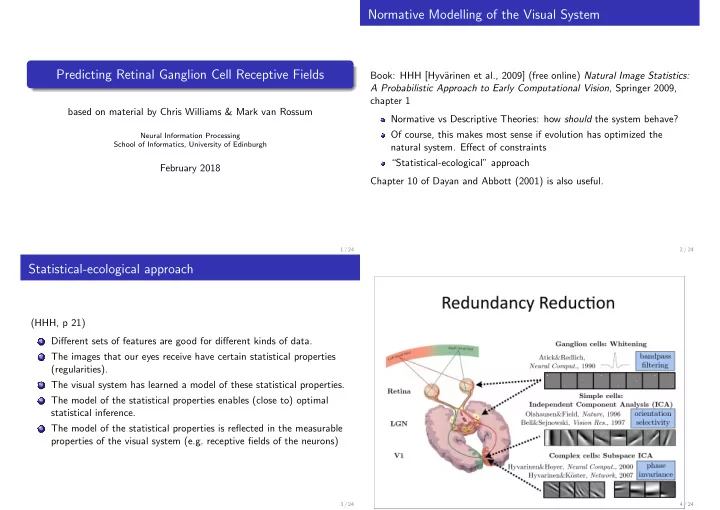
Statistical-ecological approach (HHH, p 21) 1 Different sets of features are good for different kinds of data. 2 The images that our eyes receive have certain statistical properties (regularities). 3 The visual system has learned a model of these statistical properties. 4 The model of the statistical properties enables (close to) optimal statistical inference. 5 The model of the statistical properties is reflected in the measurable properties of the visual system (e.g. receptive fields of the neurons) 3 / 24 4 / 24

  2. Mutual Informaton and Populations of Neurons Factorial Coding � H ( R ) = − p ( r ) log 2 p ( r ) d r − N log 2 ∆ r Maximization of population response entropy is achieved by and factorial coding p ( r ) = � a p ( r a ) � 1 H ( R a ) = − p ( r a ) log 2 p ( r a ) d r − log 2 ∆ r each response distribution must be optimized wrt the imposed 2 constraints We have If all neurons have the same constraints ⇒ probability equalization. � H ( R ) ≤ H ( R a ) This does not mean that each variable responds identically! a Exact factorization and probability equalization are difficult to achieve (proof, consider KL divergence) A more modest goal is decorrelation (whitening) Recall that � ( r − � r � )( r − � r � ) T � = σ 2 r I I ( R ; S ) = H ( R ) − H ( R | S ) so if noise entropy H ( R | S ) is independent of the transformation S → R , we can maximize mutual information by maximizing H ( R ) under given constraints 5 / 24 6 / 24 Second order statistics Principal Component Analysis Want � rr T � = I First order image statistics � s ( x , t ) � Subtract mean of s . Linear model (!): r = W s Second order, correlation Q ( x , x ′ , t , t ′ ) = � s ( x , t ) s ( x ′ , t ′ ) � One solution for W : PCA. Find the eigenvectors of cov ( s ) = � ss T � = Q ss and scale By Wiener-Kinchin specifying Q is equivalent to specifying s ( f ) | 2 (Wiener-Kinchin) Write Q ss = U Λ U T (where U T U = I and Λ is diagonal). Set PSD = | ˜ W = Λ − 1 / 2 U T , then � rr T � = I Gaussian approximation ⇔ Q ( x , x ′ ) ⇔ PSD First PC maximizes var ( w 1 · s ) subject to | w 1 | 2 = 1 Higher order statistics, e.g. � s ( x , t ) s ( x ′ , t ′ ) s ( x ′′ , t ′′ ) � Subsequent components: subtract previous ones and repeat procedure will be discussed later Can also be used for dimensionality reduction by removing modes with lowest eigenvalues. 7 / 24 8 / 24

  3. PCA on Natural Image Patches Whitening with PCA Figure: Hyv¨ arinen, Hurri and Hoyer (2009) If translation invariant covariance matrix, C ij = f ( | i − j | ) : eigenvectors are periodic (proof: e.g. HHH p.125). So PCA = Fourier analysis. [Hyv¨ arinen et al., 2009] To whiten:1) do PCA projections 2) scale components with inverse variance. 9 / 24 10 / 24 Generative model with PCA Importance of Fourier Phase Infomation Figure: Hyv¨ arinen, Hurri and Hoyer (2009) Left: sample images. Right: a) phase of (a) + amplitude of (b), b) v.v. [Hyv¨ arinen et al., 2009] (Method: Fourier transform image, split into magnitude and phase, s = � mix, inverse transform) k w k r k k N (0 , σ 2 P ( r ) = � k P ( r k ) = � k ) PSD contains no phase information, so second order stats miss Gaussian mix of principal components important information ... tbc. 11 / 24 12 / 24

  4. Retinal Ganglion Cell Receptive Fields Continuous-space version of the above calculation. Spatial part of the calculation only. [Atick and Redlich, 1990], also Dayan and Abbott § 4.2 Find filter D ( x ). to obtain σ r D ( κ ) | 2 ˜ � | ˜ Q ss = σ 2 | ˜ � ˜ ⇒ D ( κ ) | = r ( a ) = D ( x − a ) s ( x ) d x r Q ss � � Q rr ( a , b ) = D ( x − a ) D ( y − b ) � s ( x ) s ( y ) � d x d y Whitening filter Notice that only | ˜ D ( κ ) | is specified. Decorrelation and variance For decorrelation we require equalization do not fully specify kernel Q rr ( a , b ) = σ 2 r δ ( a , b ) Do calculations in the Fourier basis � ˜ D ( κ ) = D ( x ) exp( i κ · x ) d x 1 � ˜ D ( x ) = D ( κ ) exp( − i κ · x ) d κ 4 π 2 13 / 24 14 / 24 Filtering Input Noise Total input is s ( x ) + η ( x ), where η ( x ) is noise, reflecting image 0 + | κ | 2 ) − 1 (Field, 1987) For natural scenes ˜ Q ss ( κ ) ∝ ( κ 2 distortion, photoreceptor noise etc Filtering in the eye adds extra factor so that Optimal least-squares filter is the Wiener filter with Q ss ( κ ) = exp( − α | κ | ) ˜ ˜ κ 2 0 + | κ | 2 Q ss ( κ ) ˜ D η ( κ ) = Q ss ( κ ) + ˜ ˜ Q ηη ( κ ) Implies that | ˜ D ( κ ) | grows exponentially for large | κ | . Thus Whitening filter boosts the high frequency components (that have low power in ˜ Q ss ) D s ( κ ) = ˜ ˜ D ( κ ) ˜ D η ( κ ) � ˜ σ r Q ss ( κ ) | ˜ D s ( κ ) | = Q ss ( κ ) + ˜ ˜ Q ηη ( κ ) 15 / 24 16 / 24

  5. Figure: [Dayan and Abbott 2001] Solid curve, low noise; dashed curve, high noise Choose local, rotationally symmetric solution [Atick and Redlich, 1992] 17 / 24 18 / 24 For low noise the kernel has a bandpass character, and the predicted receptive field has a centre-surround structure This eliminates one major source of redundancy arising from strong similarity of neighbouring inputs For high noise the structure of the optimal filter is low-pass, and the RF loses its surround This averages over neighbouring inputs to extract the signal which is obscured by noise Result is not simple PCA as we have enforced spatial invariance on the filter In the retina, low light levels ≡ high noise. The predicted change matches observations [Van Nes and Bouman, 1967] 19 / 24 20 / 24

  6. Contribution of Spiking to de-correlation Further Decorrelation Analyses Spatio-temporal coding (Dong and Atick, 1995; Li, 1996). Power spectrum is 1 / f 2 but non-separable Colour opponency: red centre, green surround (and vice versa) [Atick et al., 1993] 21 / 24 22 / 24 Caveats for the Information Maximization Approach References I Atick, J. J., Li, Z., and Redlich, A. N. (1993). What does post-adaptation color appearance reveal about cortical color representation? Information maximization sets limited goals and requires strong Vision Res , 33(1):123–129. assumptions Atick, J. J. and Redlich, A. N. (1990). Towards a Theory of Early Visual Processing. Analyzes representational properties but ignores computational goals Neural Comput , 2(3):308–320. e.g. object recognition, target tracking Atick, J. J. and Redlich, A. N. (1992). Cortical processing of visual signals requires analysis beyond What does the retina know about natural scenes. Neural Comp. , 4:196–210. information transfer. V1 can have no more information about the Hyv¨ arinen, A., Hurri, J., and Hoyer, P. (2009). visual signal than the LGN, but it has many more neurons Natural Image Statistics . However, information transfer analysis does help understand mutual Spinger. selectivities: RFs with preference for high spatial frequencies are Pitkow, X. and Meister, M. (2012). Decorrelation and efficient coding by retinal ganglion cells. low-pass temporal filters, and RFs with selectivity for low spatial Nat Neurosci , 15(4):628–635. frequency act as bandpass temporal filters Van Nes, F. and Bouman, M. (1967). Spatial modulation transfer in the human eye. J Opt Soc Am , 57:401–406. 23 / 24 24 / 24

Download Presentation
Download Policy: The content available on the website is offered to you 'AS IS' for your personal information and use only. It cannot be commercialized, licensed, or distributed on other websites without prior consent from the author. To download a presentation, simply click this link. If you encounter any difficulties during the download process, it's possible that the publisher has removed the file from their server.

Recommend


More recommend