News Cool Pixar Graphics Talk Today!! Project 4 CPSC 314 Computer - PowerPoint PPT Presentation

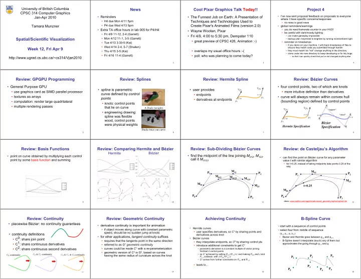
University of British Columbia News Cool Pixar Graphics Talk Today!! Project 4 CPSC 314 Computer Graphics • Reminders • The Funnest Job on Earth: A Presentation of • I've now sent proposal feedback on proposals to everyone Jan-Apr 2010 where I have specific concerns/responses • H4 due Mon 4/11 5pm Techniques and Technologies Used to • no news is good news Create Pixar's Animated Films (version 2.0) Tamara Munzner • P4 due Wed 4/13 5pm • global reminders/warnings • Extra TA office hours in lab 005 for P4/H4 • you do need framerate counter in your HUD! • Wayne Wooten, Pixar • be careful with dark/moody lighting • Fri 4/9 11-12, 2-4 (Garrett) • Fri 4/9, 4:00 to 5:30 pm, Dempster 110 • can make gameplay impossible Spatial/Scientific Visualization • Mon 4/12 11-1, 3-5 (Garrett) • backup plan: keystroke to brighten by turning more/ambient light • great preview of CPSC 426, Animation :-) • reminder on timestamps • Tue 4/13 3:30-5 (Kai) • if you demo on your machine, I will check timestamps of files to • Wed 4/14 2-4, 5-7 (Shailen) ensure they match code you submitted through handin Week 12, Fri Apr 9 • overlaps my usual office hours :-( • Thu 4/15 3-5 (Kai) • they must match! do *not* change anything in the directory • clone code into new directory to keep developing or fix tiny bugs • Fri 4/16 11-4 (Garrett) • poll: who was planning to come today? • so that I can quickly check that you've not changed anything else http://www.ugrad.cs.ubc.ca/~cs314/Vjan2010 2 3 4 Review: GPGPU Programming Review: Splines Review: Hermite Spline Review: Bézier Curves • General Purpose GPU • four control points, two of which are knots • spline is parametric • user provides • use graphics card as SIMD parallel processor • more intuitive definition than derivatives curve defined by control • endpoints • textures as arrays • curve will always remain within convex hull points • derivatives at endpoints (bounding region) defined by control points • computation: render large quadrilateral • knots: control points • multiple rendering passes that lie on curve A Duck (weight) • engineering drawing: spline was flexible wood, control points were physical weights Ducks trace out curve 5 6 7 8 Review: Basis Functions Review: Comparing Hermite and Bézier Review: Sub-Dividing Bézier Curves Review: de Casteljau’s Algorithm Hermite Bézier • find the midpoint of the line joining M 012 , M 123 . • point on curve obtained by multiplying each control • can find the point on Bézier curve for any parameter call it M 0123 point by some basis function and summing value t with similar algorithm • for t=0.25 , instead of taking midpoints take points 0.25 of the way M 12 M 12 P 1 P 2 P 2 P 1 M 012 M 0123 M 123 M 23 M 01 M 23 t=0.25 M 01 P 0 P 0 P 3 P 3 demo: www.saltire.com/applets/advanced_geometry/spline/spline.htm 9 10 11 12 Review: Continuity Review: Geometric Continuity Achieving Continuity B-Spline Curve • piecewise Bézier: no continuity guarantees • derivative continuity is important for animation • start with a sequence of control points • Hermite curves • if object moves along curve with constant parametric • select four from middle of sequence • user specifies derivatives, so C 1 by sharing points and speed, should be no sudden jump at knots (p i-2 , p i-1 , p i , p i+1 ) • continuity definitions derivatives across knot • for other applications, tangent continuity suffices • Bezier and Hermite goes between p i-2 and p i+1 • C 0 : share join point • Bezier curves • requires that the tangents point in the same direction • B-Spline doesn’t interpolate (touch) any of them but • they interpolate endpoints, so C 0 by sharing control pts • C 1 : share continuous derivatives approximates the going through p i-1 and p i • referred to as G 1 geometric continuity • introduce additional constraints to get C 1 • C 2 : share continuous second derivatives • curves could be made C 1 with a re-parameterization • parametric derivative is a constant multiple of vector joining first/last 2 control points • geometric version of C 2 is G 2 , based on curves • so C 1 achieved by setting P 0,3 =P 1,0 =J , and making P 0,2 and J and having the same radius of curvature across the knot P 2 P 6 P 1 P 1,1 collinear, with J-P 0,2 =P 1,1 -J • C 2 comes from further constraints on P 0,1 and P 1,2 • leads to... P 3 P 5 P 0 P 4 13 14 15 16

B-Spline B-Spline Geometric Modelling • by far the most popular spline used • much, much more in CPSC 424! • locality of points • C 0 , C 1 , and C 2 continuous • offered next year Spatial/Scientific Visualization demo: www.siggraph.org/education/materials/HyperGraph/modeling/splines/demoprog/curve.html 17 18 19 20 Reading Surface Graphics Surface Graphics Volume Graphics • pros • FCG Chapter 28 Spatial Field Visualization • objects explicitly defined by surface or • for some data, difficult to create polygonal mesh • fast rendering algorithms available boundary representation • voxels: discrete representation of 3D object • Chap 23 (2nd ed) • hardware acceleration cheap • volume rendering: create 2D image from 3D object • mesh of polygons • OpenGL API for programming • translate raw densities into colors and • use texture mapping for added realism • cons transparencies • discards interior of object, maintaining only the shell • different aspects of the dataset can be emphasized • operations such cutting, slicing & dissection not via changes in transfer functions possible • no artificial viewing modes such as semi- transparencies, X-ray • surface-less phenomena such as clouds, fog & gas are hard to model and represent 200 polys 1000 polys 15000 polys 21 22 23 24 Volume Graphics Isosurfaces Volume Graphics: Examples Isosurface Extraction • pros • 2D scalar fields: isolines • array of discrete point 0 1 1 3 2 samples at grid points • formidable technique for data exploration • contour plots, level sets • 3D array: voxels • topographic maps • cons 1 3 6 6 3 • find contours • 3D scalar fields: isosurfaces • rendering algorithm has high complexity! 3 7 9 7 3 • closed, continuous • special purpose hardware costly (~$3K-$10K) industrial CT - structural failure, anatomical atlas from visible security applications human (CT & MRI) datasets • determined by iso-value 2 7 8 6 2 • several methods • marching cubes is most 1 2 3 4 3 common Iso-value = 5 shockwave visualization: simulation flow around airplane wing with Navier-Stokes PDEs volumetric human head (CT scan) 25 26 27 28 MC 1: Create a Cube MC 2: Classify Each Voxel MC 3: Build An Index MC 4: Lookup Edge List • consider a cube defined by eight data values • classify each voxel according to whether lies • binary labeling of each voxel to create index • use index to access array storing list of edges • outside the surface (value > iso-surface • all 256 cases can be derived from 15 base value) cases • inside the surface (value <= iso-surface value) (i,j+1,k+1) (i+1,j+1,k+1) 10 v8 10 v7 11110100 Iso=9 inside =1 (i,j,k+1) (i+1,j,k+1) 5 v4 outside=0 5 v3 10 v5 00110000 8 v6 Iso=7 (i,j+1,k) (i+1,j+1,k) Index: 8 8 v1 v2 =inside =outside v1 v2 v3 v4 v5 v6 v7 v8 (i,j,k) (i+1,j,k) 29 30 31 32

MC 4: Example MC 5: Interpolate Triangle Vertex MC 6: Compute Normals MC 7: Render! • index = 00000001 • for each triangle edge • calculate the normal at each cube vertex • triangle 1 = a, b, c • find vertex location along edge using linear • use linear interpolation to compute the interpolation of voxel values polygon vertex normal c a i+1 i x G v v = � b x i 1 , j , k i 1 , j , k =10 + � =0 G v v = � y i , j 1 , k i , j 1 , k + � G v v = � T v [] i T=8 � � � T=5 z i , j , k 1 i , j , k 1 + � x i = + � � � ] [] � [ v i 1 v i + � � � 33 34 35 36 Rendering Pipeline Classification Transfer Functions Direct Volume Rendering • do not compute surface • data set has application-specific values • map data value to color and opacity • temperature, velocity, proton density, etc. Classify • assign these to color/opacity values to make sense of data • achieved through transfer functions 37 38 39 40 Transfer Functions Setting Transfer Functions Rendering Pipeline Light Effects • can be difficult, unintuitive, and slow • usually only consider reflected part RGB α Classify Light reflected α f α specular Light Shade RGB( f ) α ( f ) absorbed f ambient f diffuse transmitted α α Light=refl.+absorbed+trans. Light=ambient+diffuse+specular shading, I k I k I k I f = + + compositing… f a a d d s s Gordon Kindlmann 41 42 43 44 Human Tooth CT Gordon Kindlmann Rendering Pipeline Interpolation Rendering Pipeline Volume Rendering Algorithms 2D 1D • ray casting • given: • given: • image order, forward viewing Classify Classify • splatting Shade Shade • object order, backward viewing • needed: • needed: • texture mapping Interpolate Interpolate linear • object order nearest • back-to-front compositing neighbor Composite 45 46 47 48