New Methods for Time Series and Panel Econometrics 1 6 00 0 H ig - PDF document

New Methods for Time Series and Panel Econometrics 1 6 00 0 H ig h e st 1 2 00 0 H igh 8 00 0 M id 4 00 0 Po o r Po o res t 0 0 3 0 60 9 0 1 20 15 0 Average Real per C apita Income over 1960-1989 with C ountry Groupings Peter C. B. Phillips Cowles Foundation, Yale University IMF Seminar: September 29, 2003

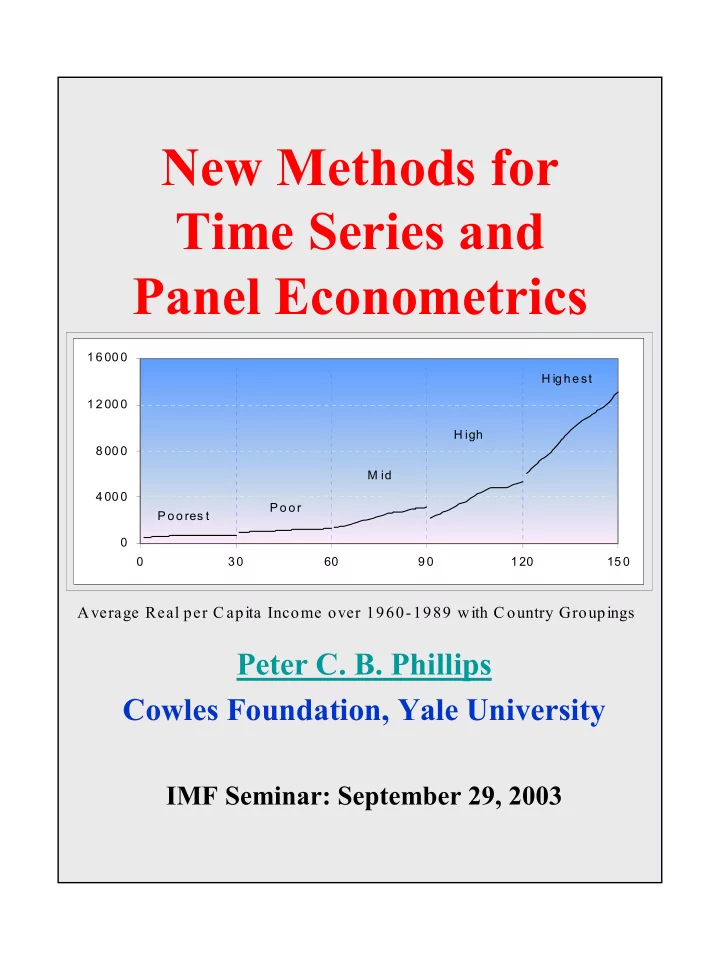
Seminar 2002 � Limitations of the Econometric Approach � Laws of Econometrics � Limits to Empirical Knowledge & Forecasting � Proximity Theorems � A Look to the Future � Online Econometric Services � Dynamic Panel Modeling � Estimation of Long Memory

Outline � Dynamic Panels with Incidental Trends & Cross Section Dependence � Bias & Inconsistency � Adjusting for Bias � Homogeneity testing � Modeling & Handling Cross Section Dependence � Nonstationary Panel Models � Unit Roots, Near unit roots, incidental trends � Testing unit roots & CSD � Cointegration & spurious regression � Applications � Growth convergence & transitions � FH savings/investment regressions � Bias corrections – PPP & demand for gas

Papers List of Relevant Papers • Phillips & Moon (1999). Linear regression limit theory for nonstationary panel data, Econometrica, 67, 1057- 1111. • Moon & Phillips (1999). Maximum likelihood estimation in panels with incidental trends. Oxford Bulletin of Economics and Statistics , 61,711–48. • Phillips & Sul (2003). Dynamic panel estimation and homogeneity testing under cross section dependence. Econometrics Journal , 6, 217-259. • Phillips & Sul (2003). Bias in Dynamic Panel Estimation with Fixed Effects, Incidental Trends and Cross Section Dependence. CFDP # 1438, Yale University • Moon, Perron & Phillips (2003). Incidental trends and the power of unit root tests. CFDP # 1435, Yale University http://cowles.econ.yale.edu/

Dynamic Panel Models Dynamic Panel Models Latent variable equation    y i , t  1  2   u i , t , u i , t  iidN  0,  i y i , t     1,1  Panel Models  , M1: y i , t  y i , t  , M2: y i , t   i  y i , t  , M3: y i , t   i   i t  y i , t Initialization 2  i N  0, 1   2      1,1    y i ,0 . O p  1    1

Dynamic Estimation Bias Estimation Bias Background & New Issues � Common autoregressive bias source & exacerbation with intercept and trend Orcutt (1949), Orcutt and Winokur (1969), Andrews (1993) � Panel autoregressive bias accentuated by pooling & effect of CS dependence Phillips & Sul (2003) � Panel autoregressive estimates inconsistent in presence of individual effects & incidental trends Nickell (1982), Neyman & Scott (1948), Moon & Phillips (1999) � Problems of Weak Instruments in IV & GMM estimation Hahn & Kuersteiner (2000), Moon & Phillips (2004)

Weak Instrument Examples Weak Instrument Examples � Applied Microeconometrics: earnings & schooling regressions Angrist & Krueger (1991, 2001) � Panel Models with Near Unit Roots Hahn & Kuersteiner (2000) Moon & Phillips (2001, 2004) 1  c y it   i  y it  1  u it T 1  c  y it   y it  1   u it T Instrument is weak because y it  2 c  y it  1   i  T y it  2  u it How does this affect inference?

Analysis of Firm Size Analysis of Firm size Gibrat’s Law (proportional effect) Z it  Z it  1  Z it  1 e it , i.e. z it  z it  1  e it Popular Empirical Formulation Sutton (1997), Hall & Mairesse (2000) z it   t  y it , y it   y it  1   it ,   1 Panel Model with Near Unit Root  g p t  c  z it   i   i T z it  1   it Moon & Phillips (2004) Implications   z it c   0 if c  0  z it  1 T

Dynamic Estimation Bias Dynamic estimation bias Models M1, M2, M3: pooled estimator T N      t  1  i  1  it  1 u it y   t  1 T  i  1 N  it  1 2 y Asymptotic Bias M2 – Nickell (1981)      G   , T    1   T  1  O  T  2  plim N     Unit Root Case M2 3   1    p lim N     T  1 also holds for heterogeneous case: N  i 2   2 N  i  1 1 2    i 2 , E  u it lim N  

Inconsistency for Model M2 Asymptotic ( N   ) Bias Function | G   , T  |   G   , T  for Model M2.

Quantiles of Pooled OLS Estimator of  = 0.9 Quantiles of pooled OLS estimator Sample Model M1 Model M2 Model M3 5% 95% 5% 95% 5% 95% N  1, T  50 0.710 0.962 0.628 0.937 0.548 0.904 N  1, T  100 0.787 0.948 0.749 0.935 0.713 0.920 N  10, T  50 0.858 0.928 0.799 0.889 0.735 0.843 N  10, T  100 0.874 0.920 0.847 0.902 0.820 0.882 N  20, T  50 0.872 0.921 0.816 0.880 0.755 0.831 N  20, T  100 0.882 0.915 0.857 0.896 0.830 0.874 N  30, T  50 0.878 0.917 0.824 0.875 0.763 0.825 N  30, T  100 0.885 0.913 0.861 0.893 0.835 0.870 N  t  1 T  pols   i  1  y it  1  y i.  1  y it  y i.   N  t  1 T  i  1  y it  1  y i.  1  2 For Model M2

Implications for Estimation of Half life implications Half-Life of Unit Shock h = 6.5,  = 0.9 Sample Model M1 Model M2 Model M3 Quantile 5% 95% 5% 95% 5% 95% N  1, T  50 2.027 18.036 1.487 10.730 1.153 6.905 N  1, T  100 2.890 13.034 2.403 10.393 2.051 8.342 N  10, T  50 4.532 9.244 3.086 5.897 2.248 4.071 N  10, T  100 5.130 8.332 4.184 6.753 3.487 5.518 N  30, T  50 5.313 8.019 3.573 5.171 2.561 3.614 N  30, T  100 5.698 7.617 4.645 6.095 3.847 4.973  h  ln0.5/ ln   pols

Panel Autoregression Panel AR density estimates density estimates 0.2 0.16 POLS PEMU 0.12 0.08 Single OLS 0.04 0 0.8 0.82 0.84 0.86 0.88 0.9 0.92 0.94 0.96 Empirical Distributions of Single Equation OLS, POLS and PEMU No Cross Section Dependence N = 20, T = 100,   0.9

Bias Reduction in Dynamic Bias reduction Panel Regression � Use Bias Correction Methods � asymptotic bias formulae – Hahn & Kuersteiner (2002), Phillips & Sul (2003) � Median Unbiased Estimation Lehmann (1959), Andrews (1993), Cermeno (1999), Phillips & Sul (2003) � use invariance property & median function of panel pooled OLS estimator � median function m     m T , N    � panel median unbiased estimator  pols  m  1  , 1 if    pemu  m  1    pols   pols  m  1  , if m   1     pols  m   1  ,  1 if 

Panel MU Estimation Panel MU Estimation � Works well …. but � Uses Gaussianity � Need to have/find median functions by simulation � Is the median function increasing? Does the inverse function exist?  pols  , m  1  m  1    pfgls  � Is it Invariant? � What about more complex models?

Model M3 Model M3 Fitted Trend: pooled estimator bias      H   , T    2 1   plim N     T  2  O  T  2  Unit Root Case M3 7 .5   1    p lim N     T  2 holds in heterogeneous error case inconsistency is > twice incidental trend case for T < 20, bias is very substantial

Inconsistency for Model M3 Asymptotic ( N   ) Bias Function | H   , T  |   H   , T  for Model M3.

Effect of Detrending Bias on Panel Data 10 y t 5 0 y t-1 -10 -5 0 5 10 -5 -10   0.90  Sample Data before Detrending ( T  4, N  1,000,   0.9,  Panel Model y it   y it  1   it ,  it  iid N  0, 1  t  1, . . . , T ; i  1, . . . , N

After Detrending 2 y t 1 0 y t-1 -2 -1 0 1 2 -1 -2 Detrended Data ( T  4, N  1,000;   0.9,    plim N       0.502,     0.53 ). Panel Model y it   y it  1   it ,  it  iid N  0, 1  t  1, . . . , T ; i  1, . . . , N

Models with Exogenous Panel AR density estimates Variables Model M4     y    y   1  Z u Asymptotic Bias M4, |  | < 1  2 A   , T            plim N  2 B   , T     plim N    ,  1   1 N Z Q Z  Z  ,  1     j Z   , t  it  j   j  0 i Z      plim   Z   1 Z   Z       plim      Z ,  1  plim     N N N

Models with Cross Section Models with cross section dependence Dependence I Model M2 + CSD K  is  st   it y it  a i   y it  1  u it , u it   s  1 where 2  over t  st  s  1, . . . , K   iid  0,  s  N N  i  1 1 2 2  si    s lim N   Asymptotic Bias M2 + CSD, |  | < 1        2 A   , T    AT plim N      2 B   , T    BT K  s  1 2   s 2   s 2  1   s   1   T  1   1  o a . s . T K T  2   s  1 2   s 2   s