neural architecture search with bayesian optimisation and
play

Neural Architecture Search with Bayesian Optimisation and Optimal - PowerPoint PPT Presentation

Neural Architecture Search with Bayesian Optimisation and Optimal Transport
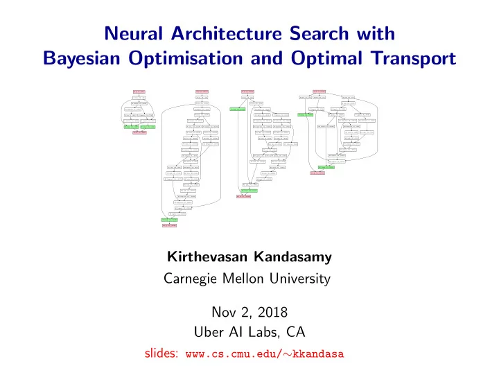
 #0 ip, 64, (28891) #0 ip, 64, (542390) #0 ip, 64, (423488) #0 ip, 64, (206092) #1 crelu, 144, (144) #1 elu, 128, (128) #1 elu, 128, (128) #3 relu, 112, (112) #2


  1. Neural Architecture Search – Prior Work Based on Reinforcement Learning: (Baker et al. 2016, Zhong et al. 2017, Zoph & Le 2017, Zoph et al. 2017) RL is more difficult than optimisation (Jiang et al. 2016) . Based on Evolutionary Algorithms: (Kitano 1990, Stanley & Miikkulainen 2002, Floreano et al. 2008, Liu et al. 2017, Miikkulainen et al. 2017, Real et al. 2017, Xie & Yuille 2017) EA works well for optimising cheap functions, but not when function evaluations are expensive. 6

  2. Neural Architecture Search – Prior Work Based on Reinforcement Learning: (Baker et al. 2016, Zhong et al. 2017, Zoph & Le 2017, Zoph et al. 2017) RL is more difficult than optimisation (Jiang et al. 2016) . Based on Evolutionary Algorithms: (Kitano 1990, Stanley & Miikkulainen 2002, Floreano et al. 2008, Liu et al. 2017, Miikkulainen et al. 2017, Real et al. 2017, Xie & Yuille 2017) EA works well for optimising cheap functions, but not when function evaluations are expensive. Other (including BO): (Swersky et al. 2014, Cortes et al. 2016, Mendoza et al. 2016, Negrinho & Gordon 2017, Jenatton et al. 2017) 6

  3. Neural Architecture Search – Prior Work Based on Reinforcement Learning: (Baker et al. 2016, Zhong et al. 2017, Zoph & Le 2017, Zoph et al. 2017) RL is more difficult than optimisation (Jiang et al. 2016) . Based on Evolutionary Algorithms: (Kitano 1990, Stanley & Miikkulainen 2002, Floreano et al. 2008, Liu et al. 2017, Miikkulainen et al. 2017, Real et al. 2017, Xie & Yuille 2017) EA works well for optimising cheap functions, but not when function evaluations are expensive. Other (including BO): (Swersky et al. 2014, Cortes et al. 2016, Mendoza et al. 2016, Negrinho & Gordon 2017, Jenatton et al. 2017) Mostly search among feed-forward structures. 6

  4. Neural Architecture Search – Prior Work Based on Reinforcement Learning: (Baker et al. 2016, Zhong et al. 2017, Zoph & Le 2017, Zoph et al. 2017) RL is more difficult than optimisation (Jiang et al. 2016) . Based on Evolutionary Algorithms: (Kitano 1990, Stanley & Miikkulainen 2002, Floreano et al. 2008, Liu et al. 2017, Miikkulainen et al. 2017, Real et al. 2017, Xie & Yuille 2017) EA works well for optimising cheap functions, but not when function evaluations are expensive. Other (including BO): (Swersky et al. 2014, Cortes et al. 2016, Mendoza et al. 2016, Negrinho & Gordon 2017, Jenatton et al. 2017) Mostly search among feed-forward structures. And a few more in the last two years ... 6

  5. Outline 1. Review ◮ Bayesian optimisation ◮ Optimal transport 2. NASBOT : Neural Architecture Search with Bayesian Optimisation & Optimal Transport ◮ OTMANN : Optimal Transport Metrics for Architectures of Neural Networks ◮ Optimising the acquisition via an evolutionary algorithm ◮ Experiments 3. Multi-fidelity optimisation in NASBOT 7

  6. Outline 1. Review ◮ Bayesian optimisation ◮ Optimal transport 2. NASBOT : Neural Architecture Search with Bayesian Optimisation & Optimal Transport ◮ OTMANN : Optimal Transport Metrics for Architectures of Neural Networks ◮ Optimising the acquisition via an evolutionary algorithm ◮ Experiments 3. Multi-fidelity optimisation in NASBOT 8

  7. Gaussian Processes ( GP ) GP ( µ, κ ): A distribution over functions from X to R . 9

  8. Gaussian Processes ( GP ) GP ( µ, κ ): A distribution over functions from X to R . Functions with no observations f ( x ) x 9

  9. Gaussian Processes ( GP ) GP ( µ, κ ): A distribution over functions from X to R . Prior GP f ( x ) x 9

  10. Gaussian Processes ( GP ) GP ( µ, κ ): A distribution over functions from X to R . Observations f ( x ) x 9

  11. Gaussian Processes ( GP ) GP ( µ, κ ): A distribution over functions from X to R . Posterior GP given observations f ( x ) x 9

  12. Gaussian Processes ( GP ) GP ( µ, κ ): A distribution over functions from X to R . Posterior GP given observations f ( x ) x Completely characterised by mean function µ : X → R , and covariance kernel κ : X × X → R . f ( x ) ∼ N ( µ t ( x ) , σ 2 After t observations, t ( x ) ). 9

  13. On the Kernel κ a.k.a covariance function, covariance kernel, covariance κ ( x , x ′ ): covariance between random variables f ( x ) and f ( x ′ ). - intuitively, κ ( x , x ′ ) is a measure of similarity between x and x ′ . 10

  14. On the Kernel κ a.k.a covariance function, covariance kernel, covariance κ ( x , x ′ ): covariance between random variables f ( x ) and f ( x ′ ). - intuitively, κ ( x , x ′ ) is a measure of similarity between x and x ′ . Some examples in Euclidean spaces κ ( x , x ′ ) = exp( − β d ( x , x ′ )) κ ( x , x ′ ) = exp( − β d ( x , x ′ ) 2 ) d ← distance between two points. E.g., d ( x , x ′ ) = � x − x ′ � 1 , or d ( x , x ′ ) = � x − x ′ � 2 . 10

  15. On the Kernel κ a.k.a covariance function, covariance kernel, covariance κ ( x , x ′ ): covariance between random variables f ( x ) and f ( x ′ ). - intuitively, κ ( x , x ′ ) is a measure of similarity between x and x ′ . Some examples in Euclidean spaces κ ( x , x ′ ) = exp( − β d ( x , x ′ )) κ ( x , x ′ ) = exp( − β d ( x , x ′ ) 2 ) d ← distance between two points. E.g., d ( x , x ′ ) = � x − x ′ � 1 , or d ( x , x ′ ) = � x − x ′ � 2 . GP Posterior: µ t ( x ) = κ ( x , X t ) ⊤ ( κ ( X t , X t ) + η 2 I ) − 1 Y σ 2 t ( x ) = κ ( x , x ) − κ ( x , X t ) ⊤ ( κ ( X t , X t ) + η 2 I ) − 1 κ ( X t , x ) . 10

  16. Bayesian Optimisation f : X → R is an expensive black-box function, accessible only via noisy evaluations. f ( x ) x 11

  17. Bayesian Optimisation f : X → R is an expensive black-box function, accessible only via noisy evaluations. f ( x ) x 11

  18. Bayesian Optimisation f : X → R is an expensive black-box function, accessible only via noisy evaluations. Let x ⋆ = argmax x f ( x ). f ( x ) f ( x ∗ ) x ∗ x 11

  19. Algorithm 1: Upper Confidence Bounds for BO Model f ∼ GP ( 0 , κ ). Gaussian Process Upper Confidence Bound ( GP-UCB ) (Srinivas et al. 2010) f ( x ) x 12

  20. Algorithm 1: Upper Confidence Bounds for BO Model f ∼ GP ( 0 , κ ). Gaussian Process Upper Confidence Bound ( GP-UCB ) (Srinivas et al. 2010) f ( x ) x 1) Compute posterior GP . 12

  21. Algorithm 1: Upper Confidence Bounds for BO Model f ∼ GP ( 0 , κ ). Gaussian Process Upper Confidence Bound ( GP-UCB ) (Srinivas et al. 2010) ϕ t = µ t − 1 + β 1 / 2 f ( x ) σ t − 1 t x 1) Compute posterior GP . 2) Construct UCB ϕ t . 12

  22. Algorithm 1: Upper Confidence Bounds for BO Model f ∼ GP ( 0 , κ ). Gaussian Process Upper Confidence Bound ( GP-UCB ) (Srinivas et al. 2010) ϕ t = µ t − 1 + β 1 / 2 f ( x ) σ t − 1 t x t x 1) Compute posterior GP . 2) Construct UCB ϕ t . 3) Choose x t = argmax x ϕ t ( x ). 12

  23. Algorithm 1: Upper Confidence Bounds for BO Model f ∼ GP ( 0 , κ ). Gaussian Process Upper Confidence Bound ( GP-UCB ) (Srinivas et al. 2010) ϕ t = µ t − 1 + β 1 / 2 f ( x ) σ t − 1 t x t x 1) Compute posterior GP . 2) Construct UCB ϕ t . 3) Choose x t = argmax x ϕ t ( x ). 4) Evaluate f at x t . 12

  24. GP-UCB (Srinivas et al. 2010) f ( x ) x 13

  25. GP-UCB (Srinivas et al. 2010) f ( x ) t = 1 x 13

  26. GP-UCB (Srinivas et al. 2010) f ( x ) t = 2 x 13

  27. GP-UCB (Srinivas et al. 2010) f ( x ) t = 3 x 13

  28. GP-UCB (Srinivas et al. 2010) f ( x ) t = 4 x 13

  29. GP-UCB (Srinivas et al. 2010) f ( x ) t = 5 x 13

  30. GP-UCB (Srinivas et al. 2010) f ( x ) t = 6 x 13

  31. GP-UCB (Srinivas et al. 2010) f ( x ) t = 7 x 13

  32. GP-UCB (Srinivas et al. 2010) f ( x ) t = 11 x 13

  33. GP-UCB (Srinivas et al. 2010) f ( x ) t = 25 x 13

  34. Theory For BO with UCB (Srinivas et al. 2010, Russo & van Roy 2014) � � � Ψ n ( X ) log( n ) f ( x ⋆ ) − max E t =1 ,..., n f ( x t ) � n Ψ n ← Maximum information gain GP with SE Kernel in d dimensions, Ψ n ( X ) ≍ vol ( X ) log( n ) d . 14

  35. Bayesian Optimisation Other criteria for selecting x t : ◮ Expected improvement (Jones et al. 1998) ◮ Thompson Sampling (Thompson 1933) ◮ Probability of improvement (Kushner et al. 1964) ◮ Entropy search (Hern´ andez-Lobato et al. 2014, Wang et al. 2017) ◮ . . . and a few more. 15

  36. Bayesian Optimisation Other criteria for selecting x t : ◮ Expected improvement (Jones et al. 1998) ◮ Thompson Sampling (Thompson 1933) ◮ Probability of improvement (Kushner et al. 1964) ◮ Entropy search (Hern´ andez-Lobato et al. 2014, Wang et al. 2017) ◮ . . . and a few more. Other Bayesian models for f : ◮ Neural networks (Snoek et al. 2015) ◮ Random Forests (Hutter 2009) 15

  37. Outline 1. Review ◮ Bayesian optimisation ◮ Optimal transport 2. NASBOT : Neural Architecture Search with Bayesian Optimisation & Optimal Transport ◮ OTMANN : Optimal Transport Metrics for Architectures of Neural Networks ◮ Optimising the acquisition via an evolutionary algorithm ◮ Experiments 3. Multi-fidelity optimisation in NASBOT 16

  38. Optimal Transport 17

  39. Optimal Transport total supply = total demand � n s i =1 s i = � n d j =1 d j . 17

  40. Optimal Transport total supply = total demand � n s i =1 s i = � n d j =1 d j . D 1 D 2 D 3 S 1 S 2 S 3 S 4 17

  41. Optimal Transport total supply = total demand � n s i =1 s i = � n d j =1 d j . D 1 D 2 D 3 S 1 C 11 C 12 C 13 S 2 S 3 S 4 17

  42. Optimal Transport total supply = total demand � n s i =1 s i = � n d j =1 d j . D 1 D 2 D 3 S 1 C 11 C 12 C 13 S 2 C 21 C 22 C 23 S 3 S 4 17

  43. Optimal Transport total supply = total demand � n s i =1 s i = � n d j =1 d j . D 1 D 2 D 3 S 1 C 11 C 12 C 13 S 2 C 21 C 22 C 23 S 3 C 31 C 32 C 33 S 4 C 41 C 42 C 43 17

  44. Optimal Transport total supply = total demand � n s i =1 s i = � n d j =1 d j . D 1 D 2 D 3 S 1 C 11 C 12 C 13 S 2 C 21 C 22 C 23 S 3 C 31 C 32 C 33 S 4 C 41 C 42 C 43 Optimal Transport Program: Let Z ∈ R n s × n d such that Z ij ← amount of mass transported from S i to D j . n s n d � � C ij Z ij = � Z , C � minimise i =1 j =1 � � subject to Z ij = s i , Z ij = d j , Z ≥ 0 i j 17

  45. Optimal Transport total supply = total demand � n s i =1 s i = � n d j =1 d j . D 1 D 2 D 3 S 1 C 11 C 12 C 13 S 2 C 21 C 22 C 23 S 3 C 31 C 32 C 33 S 4 C 41 C 42 C 43 Properties of OT ◮ OT is symmetric: solution the same if we swap sources and destinations. ◮ Connections to Wasserstein (earth mover) distances. ◮ Several efficient solvers (Peyr´ e & Cuturi 2017, Villani 2008) . ◮ OT can also be viewed as a minimum cost matching problem. 17

  46. Bayesian Optimisation for Neural Architecture Search? At each time step ϕ t = µ t − 1 + β 1 / 2 f ( x ) f ( x ) σ t − 1 t x t x x 18

  47. Bayesian Optimisation for Neural Architecture Search? At each time step ϕ t = µ t − 1 + β 1 / 2 f ( x ) f ( x ) σ t − 1 t x t x x 0: ip (100) 0: ip #0 ip, (100) (2707) 0: ip #0 ip, (100) (14456) 0: ip #0 ip, (12710) 0: ip (100) 0: ip #0 ip, (100) (2707) 0: ip #0 ip, (100) 0: ip (14456) #0 ip, (12710) (129) 1: conv7, 64 (129) 1: conv7, 64 1: conv7, 64 (64) 1: conv7, 64 (64) 1: conv3, 16 (16) 1: conv3, 16 2: conv3, 16 (64) 2: max-pool, 1 1: conv3, 16 (16) 1: conv3, 16 2: conv3, 16 (64) 2: max-pool, 1 (16) (16) #1 tanh, 8, (8) #2 logistic, 8, (8) #1 logistic, 8, (8) (64) #2 tanh, 64, (64) #3 relu, 64, (64) (16) (16) #1 tanh, 8, (8) #2 logistic, 8, (8) #1 logistic, 8, (8) (64) #2 tanh, 64, (64) #3 relu, 64, (64) 2: conv5, 128 (8192) 4: conv3, 64 (4096) 3: res3 /2, 64 (4096) 2: conv5, 128 (8192) 4: conv3, 64 (4096) 3: res3 /2, 64 (4096) 2: conv3, 8 (128) 3: conv3, 8 (128) 3: conv3, 16 4: conv5, 16 2: conv3, 8 (128) 3: conv3, 8 (128) 3: conv3, 16 4: conv5, 16 (256) (256) 3: conv3 /2, 64 7: max-pool, 1 (4096) 4: res3, 64 (256) (256) 3: conv3 /2, 64 7: max-pool, 1 (4096) 4: res3, 64 4: conv3, 32 #3 logistic, 8, (64) #4 tanh, 8, (64) (4096) (64) #2 tanh, 8, (8) #3 relu, 8, (64) 5: res3 /2, 128 #4 leaky-relu, 128, (8192) #5 logistic, 64, (4096) 4: conv3, 32 #3 logistic, 8, (64) #4 tanh, 8, (64) (4096) (64) #2 tanh, 8, (8) #3 relu, 8, (64) 5: res3 /2, 128 #4 leaky-relu, 128, (8192) #5 logistic, 64, (4096) (512) (8192) (512) (8192) 6: avg-pool, 1 (32) 5: conv5 /2, 32 (512) 5: avg-pool, 1 (128) 9: conv3, 128 (8192) (16384) 6: res3, 128 6: avg-pool, 1 (32) 5: conv5 /2, 32 (512) 5: avg-pool, 1 (128) 9: conv3, 128 (8192) (16384) 6: res3, 128 5: max-pool, 1 5: max-pool, 1 (32) #5 elu, 16, (256) #6 relu, 16, (256) 6: max-pool, 1 11: max-pool, 1 #4 softplus, 16, (256) #5 relu, 16, (256) 7: res3 /2, 256 (32768) #6 logistic, 256, (49152) #7 elu, 512, (65536) (32) #5 elu, 16, (256) #6 relu, 16, (256) 6: max-pool, 1 11: max-pool, 1 #4 softplus, 16, (256) #5 relu, 16, (256) 7: res3 /2, 256 (32768) #6 logistic, 256, (49152) #7 elu, 512, (65536) 7: fc, 32 (64) (128) 8: res3, 256 7: fc, 32 (64) (128) 8: res3, 256 6: fc, 16 (204) (65536) 6: fc, 16 (204) (65536) (51) (819) 8: fc, 64 (1228) 12: fc, 64 9: avg-pool, 1 (51) (819) 8: fc, 64 12: fc, 64 (1228) 9: avg-pool, 1 8: softmax #7 linear, (100) #6 linear, (100) (256) #1 linear, (6355) #8 linear, (6355) 8: softmax #7 linear, (100) #6 linear, (100) (256) #1 linear, (6355) #8 linear, (6355) 7: softmax (100) (129) 10: softmax 13: softmax (13107) 10: fc, 512 7: softmax (100) (129) 10: softmax 13: softmax (13107) 10: fc, 512 (1353) (1353) (1353) (1353) 9: op (14456) 11: softmax 9: op (14456) 11: softmax 8: op (100) (129) #8 op, (100) (2707) 14: op #7 op, (100) 12: op #9 op, (12710) (100) 8: op (129) #8 op, (100) 14: op (2707) #7 op, (100) 12: op #9 op, (12710) (14456) (14456) 18

  48. Bayesian Optimisation for Neural Architecture Search? At each time step ϕ t = µ t − 1 + β 1 / 2 f ( x ) f ( x ) σ t − 1 t x t x x 0: ip (100) 0: ip #0 ip, (100) (2707) 0: ip #0 ip, (100) (14456) 0: ip #0 ip, (12710) 0: ip (100) 0: ip #0 ip, (100) (2707) 0: ip #0 ip, (100) 0: ip (14456) #0 ip, (12710) (129) 1: conv7, 64 (129) 1: conv7, 64 1: conv7, 64 (64) 1: conv7, 64 (64) 1: conv3, 16 (16) 1: conv3, 16 2: conv3, 16 (64) 2: max-pool, 1 1: conv3, 16 (16) 1: conv3, 16 2: conv3, 16 (64) 2: max-pool, 1 (16) (16) #1 tanh, 8, (8) #2 logistic, 8, (8) #1 logistic, 8, (8) (64) #2 tanh, 64, (64) #3 relu, 64, (64) (16) (16) #1 tanh, 8, (8) #2 logistic, 8, (8) #1 logistic, 8, (8) (64) #2 tanh, 64, (64) #3 relu, 64, (64) 2: conv5, 128 (8192) 4: conv3, 64 (4096) 3: res3 /2, 64 (4096) 2: conv5, 128 (8192) 4: conv3, 64 (4096) 3: res3 /2, 64 (4096) 2: conv3, 8 (128) 3: conv3, 8 (128) 3: conv3, 16 4: conv5, 16 2: conv3, 8 (128) 3: conv3, 8 (128) 3: conv3, 16 4: conv5, 16 (256) (256) 3: conv3 /2, 64 7: max-pool, 1 4: res3, 64 (4096) (256) (256) 3: conv3 /2, 64 7: max-pool, 1 (4096) 4: res3, 64 4: conv3, 32 #3 logistic, 8, (64) #4 tanh, 8, (64) (4096) (64) #2 tanh, 8, (8) #3 relu, 8, (64) 5: res3 /2, 128 #4 leaky-relu, 128, (8192) #5 logistic, 64, (4096) 4: conv3, 32 #3 logistic, 8, (64) #4 tanh, 8, (64) (4096) (64) #2 tanh, 8, (8) #3 relu, 8, (64) 5: res3 /2, 128 #4 leaky-relu, 128, (8192) #5 logistic, 64, (4096) (512) (8192) (512) (8192) 6: avg-pool, 1 (32) 5: conv5 /2, 32 (512) 5: avg-pool, 1 (128) 9: conv3, 128 (8192) 6: res3, 128 (16384) 6: avg-pool, 1 (32) 5: conv5 /2, 32 (512) 5: avg-pool, 1 (128) 9: conv3, 128 (8192) (16384) 6: res3, 128 5: max-pool, 1 5: max-pool, 1 (32) #5 elu, 16, (256) #6 relu, 16, (256) 6: max-pool, 1 11: max-pool, 1 #4 softplus, 16, (256) #5 relu, 16, (256) 7: res3 /2, 256 (32768) #6 logistic, 256, (49152) #7 elu, 512, (65536) (32) #5 elu, 16, (256) #6 relu, 16, (256) 6: max-pool, 1 11: max-pool, 1 #4 softplus, 16, (256) #5 relu, 16, (256) 7: res3 /2, 256 (32768) #6 logistic, 256, (49152) #7 elu, 512, (65536) 7: fc, 32 (64) (128) 8: res3, 256 7: fc, 32 (64) (128) 8: res3, 256 6: fc, 16 (204) (65536) 6: fc, 16 (204) (65536) (51) 8: fc, 64 (819) (1228) 12: fc, 64 9: avg-pool, 1 (51) 8: fc, 64 (819) 12: fc, 64 (1228) 9: avg-pool, 1 8: softmax #7 linear, (100) #6 linear, (100) (256) #1 linear, (6355) #8 linear, (6355) 8: softmax #7 linear, (100) #6 linear, (100) (256) #1 linear, (6355) #8 linear, (6355) 7: softmax (100) (129) 10: softmax 13: softmax (13107) 10: fc, 512 7: softmax (100) (129) 10: softmax 13: softmax (13107) 10: fc, 512 (1353) (1353) (1353) (1353) 9: op (14456) 11: softmax 9: op 11: softmax (14456) 8: op (100) (129) #8 op, (100) 14: op (2707) #7 op, (100) 12: op #9 op, (12710) (100) 8: op (129) #8 op, (100) 14: op (2707) #7 op, (100) 12: op #9 op, (12710) (14456) (14456) Main challenges ◮ Define a kernel between neural network architectures. ◮ Optimise ϕ t on the space of neural networks. 18

  49. Outline 1. Review ◮ Bayesian optimisation ◮ Optimal transport 2. NASBOT : Neural Architecture Search with Bayesian Optimisation & Optimal Transport ◮ OTMANN : Optimal Transport Metrics for Architectures of Neural Networks ◮ Optimising the acquisition via an evolutionary algorithm ◮ Experiments 3. Multi-fidelity optimisation in NASBOT 19

  50. OTMANN : A distance between neural architectures (Kandasamy et al. NIPS 2018) Plan: Given a distance d , use “ κ = e − β d p ” as the kernel. 20

  51. OTMANN : A distance between neural architectures (Kandasamy et al. NIPS 2018) Plan: Given a distance d , use “ κ = e − β d p ” as the kernel. Key idea: To compute distance between architectures G 1 , G 2 , match computation (layer mass) in layers in G 1 to G 2 . 0: ip 0: ip (235) (240) Z ∈ R n 1 × n 2 . 1: conv3, 16 1: conv7, 16 (16) (16) Z ij ← amount matched between layer 2: conv3, 16 2: conv5, 32 4: conv3, 16 (256) (512) (256) i ∈ G 1 and j ∈ G 2 . 3: conv3, 32 3: conv3 /2, 16 7: max-pool, 1 (512) (256) (16) 4: conv5, 32 5: avg-pool, 1 9: conv3, 16 (1024) (32) (256) 5: max-pool, 1 6: max-pool, 1 11: max-pool, 1 (32) (16) (16) 6: fc, 16 8: fc, 16 12: fc, 16 (512) (512) (512) 7: softmax 10: softmax 13: softmax (235) (120) (120) 8: op 14: op (235) (240) 20

  52. OTMANN : A distance between neural architectures (Kandasamy et al. NIPS 2018) Plan: Given a distance d , use “ κ = e − β d p ” as the kernel. Key idea: To compute distance between architectures G 1 , G 2 , match computation (layer mass) in layers in G 1 to G 2 . 0: ip 0: ip (235) (240) Z ∈ R n 1 × n 2 . 1: conv3, 16 1: conv7, 16 (16) (16) Z ij ← amount matched between layer 2: conv3, 16 2: conv5, 32 4: conv3, 16 (256) (512) (256) i ∈ G 1 and j ∈ G 2 . 3: conv3, 32 3: conv3 /2, 16 7: max-pool, 1 (512) (256) (16) 4: conv5, 32 5: avg-pool, 1 9: conv3, 16 (1024) (32) (256) Minimise φ lmm ( Z )+ φ str ( Z )+ φ nas ( Z ) 5: max-pool, 1 6: max-pool, 1 11: max-pool, 1 (32) (16) (16) φ lmm ( Z ) : label mismatch penalty 6: fc, 16 8: fc, 16 12: fc, 16 (512) (512) (512) φ str ( Z ) : structural penalty 7: softmax 10: softmax 13: softmax (235) (120) (120) φ nas ( Z ) : non-assignment penalty 8: op 14: op (235) (240) 20

  53. The layer masses at each layer is proportional to the amount of computation at each layer 0: ip (240) Typically computed as, # incoming units × # units in layer 1: conv7, 16 (16) 2: conv5, 32 4: conv3, 16 (512) (256) 3: conv3 /2, 16 7: max-pool, 1 (256) (16) 5: avg-pool, 1 9: conv3, 16 (32) (256) 6: max-pool, 1 11: max-pool, 1 (16) (16) 8: fc, 16 12: fc, 16 (512) (512) 10: softmax 13: softmax (120) (120) 14: op (240) 21

  54. The layer masses at each layer is proportional to the amount of computation at each layer 0: ip (240) Typically computed as, # incoming units × # units in layer 1: conv7, 16 (16) 2: conv5, 32 4: conv3, 16 E.g. (512) (256) 3: conv3 /2, 16 7: max-pool, 1 ℓ m (2) = 16 × 32 = 512 . (256) (16) ℓ m (12) = (16 + 16) × 16 = 512 . 5: avg-pool, 1 9: conv3, 16 (32) (256) 6: max-pool, 1 11: max-pool, 1 (16) (16) 8: fc, 16 12: fc, 16 (512) (512) 10: softmax 13: softmax (120) (120) 14: op (240) 21

  55. The layer masses at each layer is proportional to the amount of computation at each layer 0: ip (240) Typically computed as, # incoming units × # units in layer 1: conv7, 16 (16) 2: conv5, 32 4: conv3, 16 E.g. (512) (256) 3: conv3 /2, 16 7: max-pool, 1 ℓ m (2) = 16 × 32 = 512 . (256) (16) ℓ m (12) = (16 + 16) × 16 = 512 . 5: avg-pool, 1 9: conv3, 16 (32) (256) 6: max-pool, 1 11: max-pool, 1 (16) (16) A few exceptions: - input, output layers 8: fc, 16 12: fc, 16 (512) (512) - softmax/linear layers 10: softmax 13: softmax - fully connected layers in CNNs (120) (120) 14: op (240) 21

  56. Label mismatch penalty Define M , 0: ip 0: ip (235) (240) c3 c5 mp ap fc 1: conv3, 16 1: conv7, 16 (16) (16) 0 0 . 2 c3 2: conv3, 16 2: conv5, 32 4: conv3, 16 (256) (512) (256) 0 . 2 0 c5 0 0 . 25 3: conv3, 32 3: conv3 /2, 16 7: max-pool, 1 ap (512) (256) (16) 0 . 25 0 mp 4: conv5, 32 5: avg-pool, 1 9: conv3, 16 (1024) (32) (256) 0 fc 5: max-pool, 1 6: max-pool, 1 11: max-pool, 1 (32) (16) (16) 6: fc, 16 8: fc, 16 12: fc, 16 (512) (512) (512) 7: softmax 10: softmax 13: softmax (235) (120) (120) 8: op 14: op (235) (240) 22

  57. Label mismatch penalty Define M , 0: ip 0: ip (235) (240) c3 c5 mp ap fc 1: conv3, 16 1: conv7, 16 (16) (16) 0 0 . 2 c3 2: conv3, 16 2: conv5, 32 4: conv3, 16 (256) (512) (256) 0 . 2 0 c5 0 0 . 25 3: conv3, 32 3: conv3 /2, 16 7: max-pool, 1 ap (512) (256) (16) 0 . 25 0 mp 4: conv5, 32 5: avg-pool, 1 9: conv3, 16 (1024) (32) (256) 0 fc 5: max-pool, 1 6: max-pool, 1 11: max-pool, 1 (32) (16) (16) Define C lmm ∈ R n 1 × n 2 where, 6: fc, 16 8: fc, 16 12: fc, 16 (512) (512) (512) 7: softmax 10: softmax 13: softmax C lmm ( i , j ) = M ( ℓℓ ( i ) , ℓℓ ( j )) . (235) (120) (120) 8: op 14: op (235) (240) 22

  58. Label mismatch penalty Define M , 0: ip 0: ip (235) (240) c3 c5 mp ap fc 1: conv3, 16 1: conv7, 16 (16) (16) 0 0 . 2 c3 2: conv3, 16 2: conv5, 32 4: conv3, 16 (256) (512) (256) 0 . 2 0 c5 0 0 . 25 3: conv3, 32 3: conv3 /2, 16 7: max-pool, 1 ap (512) (256) (16) 0 . 25 0 mp 4: conv5, 32 5: avg-pool, 1 9: conv3, 16 (1024) (32) (256) 0 fc 5: max-pool, 1 6: max-pool, 1 11: max-pool, 1 (32) (16) (16) Define C lmm ∈ R n 1 × n 2 where, 6: fc, 16 8: fc, 16 12: fc, 16 (512) (512) (512) 7: softmax 10: softmax 13: softmax C lmm ( i , j ) = M ( ℓℓ ( i ) , ℓℓ ( j )) . (235) (120) (120) 8: op 14: op (235) (240) Label mismatch penalty, φ lmm ( Z ) = � Z , C lmm � . 22

  59. Structural Penalty δ sp op ( i ) , δ lp op ( i ) , δ rw op ( i ) ← shortest, longest, random walk path lenghts from layer i to output. 0: ip 0: ip (235) (240) 1: conv3, 16 1: conv7, 16 (16) (16) 2: conv3, 16 2: conv5, 32 4: conv3, 16 (256) (512) (256) 3: conv3, 32 3: conv3 /2, 16 7: max-pool, 1 (512) (256) (16) 4: conv5, 32 5: avg-pool, 1 9: conv3, 16 (1024) (32) (256) 5: max-pool, 1 6: max-pool, 1 11: max-pool, 1 (32) (16) (16) 6: fc, 16 8: fc, 16 12: fc, 16 (512) (512) (512) 7: softmax 10: softmax 13: softmax (235) (120) (120) 8: op 14: op (235) (240) 23

  60. Structural Penalty δ sp op ( i ) , δ lp op ( i ) , δ rw op ( i ) ← shortest, longest, random walk path lenghts from layer i to output. E.g. (in right network): δ sp op (1) = 5, 0: ip 0: ip (235) (240) δ lp op (1) = 7, δ rw op (1) = 5 . 67. 1: conv3, 16 1: conv7, 16 (16) (16) 2: conv3, 16 2: conv5, 32 4: conv3, 16 (256) (512) (256) 3: conv3, 32 3: conv3 /2, 16 7: max-pool, 1 (512) (256) (16) 4: conv5, 32 5: avg-pool, 1 9: conv3, 16 (1024) (32) (256) 5: max-pool, 1 6: max-pool, 1 11: max-pool, 1 (32) (16) (16) 6: fc, 16 8: fc, 16 12: fc, 16 (512) (512) (512) 7: softmax 10: softmax 13: softmax (235) (120) (120) 8: op 14: op (235) (240) 23

  61. Structural Penalty δ sp op ( i ) , δ lp op ( i ) , δ rw op ( i ) ← shortest, longest, random walk path lenghts from layer i to output. Similarly define δ sp ip ( i ) , δ lp ip ( i ) , δ rw ip ( i ) from input to layer i . E.g. (in right network): δ sp op (1) = 5, 0: ip 0: ip (235) (240) δ lp op (1) = 7, δ rw op (1) = 5 . 67. 1: conv3, 16 1: conv7, 16 (16) (16) 2: conv3, 16 2: conv5, 32 4: conv3, 16 (256) (512) (256) 3: conv3, 32 3: conv3 /2, 16 7: max-pool, 1 (512) (256) (16) 4: conv5, 32 5: avg-pool, 1 9: conv3, 16 (1024) (32) (256) 5: max-pool, 1 6: max-pool, 1 11: max-pool, 1 (32) (16) (16) 6: fc, 16 8: fc, 16 12: fc, 16 (512) (512) (512) 7: softmax 10: softmax 13: softmax (235) (120) (120) 8: op 14: op (235) (240) 23

  62. Structural Penalty δ sp op ( i ) , δ lp op ( i ) , δ rw op ( i ) ← shortest, longest, random walk path lenghts from layer i to output. Similarly define δ sp ip ( i ) , δ lp ip ( i ) , δ rw ip ( i ) from input to layer i . E.g. (in right network): δ sp op (1) = 5, 0: ip 0: ip (235) (240) δ lp op (1) = 7, δ rw op (1) = 5 . 67. 1: conv3, 16 1: conv7, 16 (16) (16) 2: conv3, 16 2: conv5, 32 4: conv3, 16 (256) (512) (256) Let C str ∈ R n 1 × n 2 where, 3: conv3, 32 3: conv3 /2, 16 7: max-pool, 1 (512) (256) (16) C str ( i , j ) = 1 � � | δ s t ( i ) − δ s t ( j ) | . 4: conv5, 32 5: avg-pool, 1 9: conv3, 16 (1024) (32) (256) 6 s t 5: max-pool, 1 6: max-pool, 1 11: max-pool, 1 (32) (16) (16) s ∈ { sp, lp, rw } , t ∈ { ip,op } 6: fc, 16 8: fc, 16 12: fc, 16 (512) (512) (512) 7: softmax 10: softmax 13: softmax (235) (120) (120) 8: op 14: op (235) (240) 23

  63. Structural Penalty δ sp op ( i ) , δ lp op ( i ) , δ rw op ( i ) ← shortest, longest, random walk path lenghts from layer i to output. Similarly define δ sp ip ( i ) , δ lp ip ( i ) , δ rw ip ( i ) from input to layer i . E.g. (in right network): δ sp op (1) = 5, 0: ip 0: ip (235) (240) δ lp op (1) = 7, δ rw op (1) = 5 . 67. 1: conv3, 16 1: conv7, 16 (16) (16) 2: conv3, 16 2: conv5, 32 4: conv3, 16 (256) (512) (256) Let C str ∈ R n 1 × n 2 where, 3: conv3, 32 3: conv3 /2, 16 7: max-pool, 1 (512) (256) (16) C str ( i , j ) = 1 � � | δ s t ( i ) − δ s t ( j ) | . 4: conv5, 32 5: avg-pool, 1 9: conv3, 16 (1024) (32) (256) 6 s t 5: max-pool, 1 6: max-pool, 1 11: max-pool, 1 (32) (16) (16) s ∈ { sp, lp, rw } , t ∈ { ip,op } 6: fc, 16 8: fc, 16 12: fc, 16 (512) (512) (512) 7: softmax 10: softmax 13: softmax (235) (120) (120) Structural penalty, 8: op 14: op (235) (240) φ str ( Z ) = � Z , C str � . 23

  64. Non-assignment penalty The non-assignment penalty is the amount of mass unmatched in both networks, � � � � � � � � φ nas ( Z ) = ℓ m ( i ) − + ℓ m ( j ) − Z ij Z ij . i ∈L 1 j ∈L 2 j ∈L 2 i ∈L 1 The cost per unit for unassigned mass is 1. 24

  65. Optimal Transport total supply = total demand � n s i =1 s i = � n d j =1 d j . D 1 D 2 D 3 S 1 C 11 C 12 C 13 S 2 C 21 C 22 C 23 S 3 C 31 C 32 C 33 S 4 C 41 C 42 C 43 Optimal Transport Program: Let Z ∈ R n s × n d such that Z ij ← amount of mass transported from S i to D j . n s n d � � C ij Z ij = � Z , C � minimise i =1 j =1 � � Z ij = s i , Z ij = d i , Z ≥ 0 subject to i j 25

  66. Computing OTMANN via Optimal Transport Introduce sink layers with mass equal to total mass of other net- 0: ip 0: ip (235) (240) work. Unit cost for matching sink 1: conv3, 16 1: conv7, 16 (16) (16) nodes is 0. 2: conv3, 16 2: conv5, 32 4: conv3, 16 (256) (512) (256) 3: conv3, 32 3: conv3 /2, 16 7: max-pool, 1 (512) (256) (16) 4: conv5, 32 5: avg-pool, 1 9: conv3, 16 (1024) (32) (256) 5: max-pool, 1 6: max-pool, 1 11: max-pool, 1 (32) (16) (16) 6: fc, 16 8: fc, 16 12: fc, 16 (512) (512) (512) 7: softmax 10: softmax 13: softmax (235) (120) (120) 8: op 14: op (235) (240) sink_1 (3120) 26

  67. Computing OTMANN via Optimal Transport Introduce sink layers with mass equal to total mass of other net- 0: ip 0: ip (235) (240) work. Unit cost for matching sink 1: conv3, 16 1: conv7, 16 (16) (16) nodes is 0. 2: conv3, 16 2: conv5, 32 4: conv3, 16 (256) (512) (256) OT variable Z ′ and cost matrix C ′ , 3: conv3, 32 3: conv3 /2, 16 7: max-pool, 1 (512) (256) (16) C ′ , Z ′ ∈ R ( n 1 +1) × ( n 2 +1) . 4: conv5, 32 5: avg-pool, 1 9: conv3, 16 (1024) (32) (256) 5: max-pool, 1 6: max-pool, 1 11: max-pool, 1 (32) (16) (16) 6: fc, 16 8: fc, 16 12: fc, 16 (512) (512) (512) 7: softmax 10: softmax 13: softmax (235) (120) (120) 8: op 14: op (235) (240) sink_1 (3120) 26

  68. Computing OTMANN via Optimal Transport Introduce sink layers with mass equal to total mass of other net- 0: ip 0: ip (235) (240) work. Unit cost for matching sink 1: conv3, 16 1: conv7, 16 (16) (16) nodes is 0. 2: conv3, 16 2: conv5, 32 4: conv3, 16 (256) (512) (256) OT variable Z ′ and cost matrix C ′ , 3: conv3, 32 3: conv3 /2, 16 7: max-pool, 1 (512) (256) (16) C ′ , Z ′ ∈ R ( n 1 +1) × ( n 2 +1) . 4: conv5, 32 5: avg-pool, 1 9: conv3, 16 (1024) (32) (256) For i ≤ n 1 , j ≤ n 2 , 5: max-pool, 1 6: max-pool, 1 11: max-pool, 1 (32) (16) (16) C ′ ( i , j ) = C lmm ( i , j ) + C str ( i , j ) 6: fc, 16 8: fc, 16 12: fc, 16 (512) (512) (512) C ′ looks as follows, 7: softmax 10: softmax 13: softmax (235) (120) (120) 1 8: op 14: op (235) (240) . . C lmm + C str . sink_1 (3120) 1 1 · · · 1 0 26

  69. Theoretical Properties of OTMANN (Kandasamy et al. NIPS 2018) 1. It can be computed via an optimal transport scheme. 2. Under mild regularity conditions, it is a pseudo-distance. That is, given neural networks G 1 , G 2 , G 3 , ◮ d ( G 1 , G 2 ) ≥ 0. ◮ d ( G 1 , G 2 ) = d ( G 2 , G 1 ). ◮ d ( G 1 , G 3 ) ≤ d ( G 1 , G 2 ) + d ( G 2 , G 3 ). 27

  70. Theoretical Properties of OTMANN (Kandasamy et al. NIPS 2018) 1. It can be computed via an optimal transport scheme. 2. Under mild regularity conditions, it is a pseudo-distance. That is, given neural networks G 1 , G 2 , G 3 , ◮ d ( G 1 , G 2 ) ≥ 0. ◮ d ( G 1 , G 2 ) = d ( G 2 , G 1 ). ◮ d ( G 1 , G 3 ) ≤ d ( G 1 , G 2 ) + d ( G 2 , G 3 ). From distance to kernel: Given OTMANN distance d , use κ = e − β d as the “kernel”. 27

  71. OTMANN : Illustration with tSNE Embeddings #0 ip, #0 ip, #0 ip, #0 ip, (110) [1] (113) [1] j (8179) [1] (100) [1] a b #1 res5, 16, #1 conv3, 18, #1 conv7, 72, (16) [1] (18) [1] (72) [1] #1 conv3, 16, (16) [1] #2 conv3, 18, #6 avg-pool, #3 conv3, 63, #4 conv3, 81, #5 conv3, 71, #2 conv3, 9, #3 res3, 9, (324) [1] (72) [1] (4536) [1, /2] (5832) [1] (5112) [1] #2 conv3, 16, (144) [1] (144) [1] (256) [1] c #3 conv3, 32, #9 max-pool, #10 max-pool, #11 max-pool, #6 conv3, 32, #4 avg-pool, (576) [1] #3 conv3, 32, (576) [1] (16) [1] (63) [2] (81) [1] (71) [1] (512) [1] #7 avg-pool, #5 avg-pool, #4 avg-pool, #5 max-pool, #2 conv5, 144, #14 conv3, 110, #16 conv3, 142, #17 conv3, 126, (32) [1] (16) [1] (18) [1] (32) [1] (10368) [1, /2] (8910) [2, /2] (21584) [2] (8946) [2] #4 max-pool, (32) [1] #8 fc, 20, #6 fc, 14, #7 fc, 14, #8 fc, 16, #7 avg-pool, #12 avg-pool, #19 conv3, 87, #15 avg-pool, #20 max-pool, #21 max-pool, (70) [2] (44) [2] (51) [2] (144) [2] (72) [2] (9570) [4] (81) [2] (142) [2] (126) [2] #5 fc, 16, (128) [2] (51) [2] #9 softmax, #10 softmax, #11 softmax, #8 fc, 79, #18 fc, 48, #22 fc, 63, #23 fc, 63, #24 fc, 55, #9 fc, 18, (37) [x] (37) [x] (37) [x] (1137) [2] (1036) [4] (1839) [4] (1304) [4] (693) [4] #6 softmax, (36) [x] (100) [x] #10 softmax, #12 op, #13 softmax, #25 softmax, #26 softmax, #7 op, (110) [x] (113) [x] (2726) [x] (2726) [x] (2726) [x] (100) [x] #11 op, #27 op, (110) [x] (8179) [x] #0 ip, (5427) [1] #0 ip, (93661) [1] #0 ip, k #0 ip, (76459) [1] #1 conv7, 64, (63764) [1] (64) [1] d f #1 conv3, 64, (64) [1] #1 conv3, 56, #1 conv3, 56, (56) [1] #4 conv3, 64, #5 conv3, 64, #7 avg-pool, #3 conv3, 56, #6 avg-pool, t-SNE: OTMANN Distance (56) [1] e (4096) [1] (4096) [1] (64) [1] (3584) [1, /2] (64) [1] #2 conv3, 64, #2 conv3, 56, (4096) [1] #2 conv3, 63, j (3136) [1] (3528) [1] #11 avg-pool, #13 max-pool, #15 avg-pool, #14 avg-pool, #2 conv7, 128, k (64) [1] (64) [1] (64) [2] (64) [2] (8192) [1, /2] #3 max-pool, (64) [1] #4 max-pool, #3 avg-pool, #3 max-pool, (63) [1] (56) [1] #12 avg-pool, #17 conv3, 128, #19 conv3, 128, #20 res3, 56, #8 max-pool, (56) [1] (64) [1] (8192) [2] (16384) [2] (3584) [4] (128) [2] #4 conv5, 144, 4 (9216) [2] #6 conv3, 112, #5 conv3, 112, #4 conv3, 112, (7056) [2] (6272) [2] #18 max-pool, #21 max-pool, #23 max-pool, #10 max-pool, #24 fc, 56, (6272) [2] (64) [2] (192) [2] (128) [2] (56) [2] (1030) [4] i #5 conv7, 144, #6 conv7, 128, (20736) [2] (18432) [2] #5 conv3, 128, #8 conv3, 128, #7 conv3, 128, (14336) [2] (14336) [2] (14336) [2] #22 fc, 64, #26 fc, 64, #9 fc, 63, (409) [4] (2816) [4] (806) [2] #7 max-pool, #9 max-pool, 2 #6 max-pool, (144) [2] (128) [2] #10 max-pool, #9 max-pool, (128) [2] (128) [2] #25 softmax, #27 softmax, #16 softmax, (128) [2] (1809) [x] (1809) [x] (1809) [x] #0 ip, (20613) [1] #8 max-pool, #11 conv3, 128, #0 ip, (144) [2] (34816) [4] #11 conv3, 128, (28787) [1] #7 conv3, 128, (16384) [4] #28 op, (16384) [4] (5427) [x] h #1 conv3, 56, #10 conv3, 128, #13 conv3, 128, #1 conv3, 56, n (56) [1] (18432) [4] (16384) [4] #12 conv3, 128, (56) [1] n #8 conv3, 128, 0 (16384) [4] (16384) [4] g #2 max-pool, #3 max-pool, m (56) [1] (56) [1] #12 conv3, 128, #15 conv3, 128, #2 max-pool, #3 max-pool, #9 conv3, 128, (16384) [4] (16384) [4] #13 conv3, 112, (56) [1] (56) [1] (16384) [4] (28672) [4] #4 conv5, 63, #5 avg-pool, #6 max-pool, (3528) [2, /2] (56) [2] (56) [2] #14 conv3, 128, #17 max-pool, m #4 conv5, 63, c (16384) [4] (128) [4] #14 conv3, 112, (3528) [2, /2] #10 avg-pool, (12544) [4] 2 (128) [4] #7 res5, 62, #8 conv5, 56, b #16 max-pool, #19 conv3, 256, #6 res5, 62, (3906) [4] (6272) [4] a (128) [4] (32768) [8] #15 avg-pool, (3906) [4] #11 conv3, 256, (112) [4] (32768) [8] #10 res7, 92, #11 max-pool, #9 conv5, 56, #18 conv3, 256, #20 conv3, 288, (5704) [4] (56) [4] (3136) [4] #9 res7, 92, #5 avg-pool, #12 conv3, 256, (32768) [8] (73728) [8] #16 conv3, 256, (5704) [4] (56) [2] (65536) [8] (28672) [8] #13 res3, 128, #14 avg-pool, #12 avg-pool, 4 (11776) [4, /2] (56) [8] (56) [4] #21 max-pool, #13 res3, 128, #7 conv5, 56, #8 conv5, 56, (544) [8] #17 conv3, 288, (11776) [4, /2] (3136) [4] (3136) [4] #13 max-pool, (73728) [8] (256) [8] #16 res3, 128, #17 conv3, 128, #15 avg-pool, (16384) [8] (16384) [8] (56) [8] #22 conv3, 512, #16 res3, 128, #17 conv3, 128, #11 avg-pool, #10 avg-pool, (278528) [16] #18 max-pool, (16384) [8] (16384) [8] (56) [4] (56) [4] #14 conv3, 576, (288) [8] (147456) [16] #19 avg-pool, #20 res3, 224, #18 avg-pool, 6 #23 conv3, 512, (128) [8] (28672) [8, /2] (56) [16] (262144) [16] #19 res3, 224, #20 res3, 224, #14 avg-pool, #12 avg-pool, #15 conv3, 512, #19 conv3, 648, (28672) [8, /2] (41216) [8, /2] (56) [8] (56) [4] (294912) [16] (186624) [16] #22 res3, 256, #23 conv3, 224, #21 fc, 392, (32768) [16] (50176) [16] (2195) [32] #24 max-pool, #22 res3, 256, #23 res3, 256, #24 avg-pool, #15 avg-pool, #16 max-pool, (512) [16] #20 conv3, 512, (57344) [16] (57344) [16] (280) [16] (56) [8] (331776) [16] (512) [16] #25 max-pool, #26 avg-pool, #24 softmax, (256) [16] (280) [16] (6871) [x] 8 #25 conv5, 128, #26 max-pool, #27 max-pool, #28 fc, 448, #18 avg-pool, (65536) [32] #21 max-pool, (256) [16] (256) [16] (12544) [32] (56) [16] #17 fc, 128, (512) [16] d (6553) [32] f #27 fc, 448, #28 fc, 448, #26 fc, 128, #29 fc, 448, #21 fc, 448, (11468) [32] (12544) [32] (1638) [32] #22 fc, 128, (22937) [32] (2508) [32] e #18 fc, 256, (6553) [32] (3276) [x] #29 softmax, #30 softmax, (6871) [x] (6871) [x] #27 fc, 256, #31 softmax, #30 softmax, #25 softmax, 10 #19 fc, 512, (3276) [x] #23 fc, 256, (9595) [x] (9595) [x] (9595) [x] (13107) [x] (3276) [x] #31 op, (20613) [x] 10 8 6 4 2 0 2 #28 fc, 512, #32 op, (13107) [x] #24 fc, 512, (28787) [x] #20 softmax, (13107) [x] (63764) [x] #0 ip, #29 softmax, (459) [1] (93661) [x] #25 softmax, #21 op, (76459) [x] i (63764) [x] #30 op, #1 conv3, 16, #2 conv3, 16, (16) [1] (16) [1] (93661) [x] #26 op, (76459) [x] #5 avg-pool, #3 res5, 16, #4 conv3, 16, (16) [1] (256) [1] (256) [1] #0 ip, (264) [1] #0 ip, (284) [1] h #7 conv5, 32, #9 conv3, 32, #6 conv3, 16, (512) [1] (512) [1] (256) [1] g #1 conv3, 16, #2 conv3, 18, (16) [1] (18) [1] #1 conv3, 18, #2 conv3, 20, (18) [1] (20) [1] #8 res3, 32, #11 conv3, 32, #13 avg-pool, #10 avg-pool, #3 conv3, 16, #6 conv3, 36, (512) [1] (1024) [1] (32) [1] (16) [1] (256) [1] (648) [1] #4 conv3, 41, #3 conv3, 18, #6 conv3, 41, (738) [1] (324) [1] (820) [1] #12 avg-pool, #15 avg-pool, #14 avg-pool, #16 fc, 32, #4 conv3, 36, #5 max-pool, #8 avg-pool, #7 max-pool, (32) [1] (32) [1] (32) [1] (153) [2] (576) [1] (16) [1] (16) [1] (16) [1] #5 avg-pool, #8 avg-pool, #7 max-pool, #11 max-pool, (18) [1] (18) [1] (18) [1] (41) [1] #18 fc, 36, #17 fc, 36, (288) [2] (115) [2] #9 max-pool, #10 max-pool, #13 fc, 28, #12 max-pool, (36) [1] (36) [1] (134) [2] (36) [1] #9 max-pool, #12 fc, 32, #14 fc, 25, (41) [1] (172) [2] (102) [2] #20 fc, 36, #19 fc, 36, (259) [x] (129) [x] #14 fc, 28, #15 fc, 28, #11 fc, 28, #17 fc, 32, #16 fc, 28, (100) [2] (100) [2] (44) [2] (89) [x] (100) [2] #13 fc, 25, #10 fc, 32, #15 fc, 25, #18 fc, 19, (102) [2] (57) [2] (80) [x] (47) [x] #21 fc, 36, #19 fc, 28, #18 fc, 32, #21 fc, 28, #20 fc, 25, (129) [x] (78) [x] (89) [x] (168) [x] (70) [x] #17 fc, 22, #16 fc, 19, #19 fc, 22, (55) [x] (47) [x] (125) [x] #22 softmax, (459) [x] #23 softmax, #22 softmax, #25 softmax, #24 softmax, (66) [x] (66) [x] (66) [x] (66) [x] #21 softmax, #20 softmax, #23 softmax, #22 softmax, (71) [x] (71) [x] (71) [x] (71) [x] #23 op, (459) [x] #26 op, (264) [x] #24 op, (284) [x] 28

  72. OTMANN correlates with cross validation performance 29

  73. Outline 1. Review ◮ Bayesian optimisation ◮ Optimal transport 2. NASBOT : Neural Architecture Search with Bayesian Optimisation & Optimal Transport ◮ OTMANN : Optimal Transport Metrics for Architectures of Neural Networks ◮ Optimising the acquisition via an evolutionary algorithm ◮ Experiments 3. Multi-fidelity optimisation in NASBOT 30

  74. Optimising the acquisition via an Evolutionary Algorithm EA navigates the search space by applying a sequence of local modifiers to the points already evaluated. 31

  75. Optimising the acquisition via an Evolutionary Algorithm EA navigates the search space by applying a sequence of local modifiers to the points already evaluated. Each modifier: ◮ Takes a network, modifies and returns a new one. ◮ Each modifier can change the number of units in each layer, add/delte layers, or modify the architecture of the network. 31

  76. Optimising the acquisition via an Evolutionary Algorithm EA navigates the search space by applying a sequence of local modifiers to the points already evaluated. Each modifier: ◮ Takes a network, modifies and returns a new one. ◮ Each modifier can change the number of units in each layer, add/delte layers, or modify the architecture of the network. ◮ Care must be taken to ensure that the resulting networks are still “valid”. 31

  77. inc single #0 ip #0 ip #1 conv7 #1 conv7 64 64 #2 max-pool #2 max-pool #3 conv3 #3 conv3 64 64 #4 conv3 #4 conv3 128 128 #5 conv3 #5 conv3 256 288 #6 conv3 #6 conv3 512 512 #7 avg-pool #7 avg-pool #8 fc #8 fc 1024 1024 #9 softmax #9 softmax #10 op #10 op Similarly define dec single 32

  78. inc en masse #0 ip #0 ip #1 conv7 #1 conv7 64 64 #2 max-pool #2 max-pool #3 conv3 #3 conv3 64 64 #4 conv3 #4 conv3 128 128 #5 conv3 #5 conv3 256 288 #6 conv3 #6 conv3 512 576 #7 avg-pool #7 avg-pool #8 fc #8 fc 1024 1152 #9 softmax #9 softmax #10 op #10 op Similarly define dec en masse 33

  79. remove layer #0 ip #0 ip #1 conv7 64 #1 conv7 64 #2 max-pool #2 max-pool #3 conv3 64 #3 conv3 64 #4 conv3 128 #4 conv3 256 #5 conv3 256 #5 conv3 512 #6 conv3 512 #6 max-pool #7 avg-pool #7 fc 1024 #8 fc 1024 #8 softmax #9 softmax #9 op #10 op 34

  80. wedge layer #0 ip #0 ip #1 conv7 64 #1 conv7 64 #2 max-pool #2 max-pool #3 conv7 64 #3 conv3 64 #4 conv3 64 #4 conv3 128 #5 conv3 128 #5 conv3 256 #6 conv3 256 #6 conv3 512 #7 conv3 512 #7 avg-pool #8 avg-pool #8 fc 1024 #9 fc 1024 #9 softmax #10 softmax #10 op #11 op 35

  81. swap label #0 ip #0 ip #1 conv7 #1 conv7 64 64 #2 max-pool #2 max-pool #3 conv3 #3 conv3 64 64 #4 conv3 #4 conv3 128 128 #5 conv3 #5 conv3 256 256 #6 conv3 #6 conv5 512 512 #7 avg-pool #7 avg-pool #8 fc #8 fc 1024 1024 #9 softmax #9 softmax #10 op #10 op 36

  82. dup path #0 ip #0 ip #1 conv7 #1 conv7 #2 conv7 64 64 64 #2 max-pool #3 max-pool #4 max-pool #3 conv3 #5 conv3 #6 conv3 64 64 64 #4 conv3 #7 conv3 #8 conv3 128 128 128 #5 conv3 #9 conv3 #10 conv3 256 256 256 #6 conv3 #11 conv3 512 512 #7 avg-pool #12 avg-pool #8 fc #13 fc 1024 1024 #9 softmax #14 softmax #10 op #15 op 37

  83. skip #0 ip #0 ip #1 conv7 #1 conv7 64 64 #2 max-pool #2 max-pool #3 conv3 #3 conv3 64 64 #4 conv3 #4 conv3 64 64 #5 conv3 #5 conv3 128 128 #6 conv3 #6 conv3 128 128 #7 conv3 #7 conv3 256 256 #8 conv3 #8 conv3 256 256 #9 avg-pool #9 avg-pool #10 fc #10 fc 512 512 #11 softmax #11 softmax #12 op #12 op 38

  84. Optimising the acquisition via EA Goal: optimise the acquisition (e.g. UCB, EI etc.) 39

  85. Optimising the acquisition via EA Goal: optimise the acquisition (e.g. UCB, EI etc.) ◮ Evaluate the acquisition on an initial pool of networks. 39

  86. Optimising the acquisition via EA Goal: optimise the acquisition (e.g. UCB, EI etc.) ◮ Evaluate the acquisition on an initial pool of networks. ◮ Stochastically select those that have a high acquisition value and apply modifiers to generate a pool of candidates. 39

  87. Optimising the acquisition via EA Goal: optimise the acquisition (e.g. UCB, EI etc.) ◮ Evaluate the acquisition on an initial pool of networks. ◮ Stochastically select those that have a high acquisition value and apply modifiers to generate a pool of candidates. ◮ Evaluate the acquisition on those candidates and repeat. 39

  88. Neural Architecture Search via Bayesian Optimisation At each time step ϕ t = µ t − 1 + β 1 / 2 f ( x ) f ( x ) σ t − 1 t x t x x 0: ip 0: ip 0: ip (100) (129) 0: ip #0 ip, (100) (2707) 0: ip #0 ip, (100) (14456) #0 ip, (12710) 0: ip (100) 0: ip (129) #0 ip, (100) 0: ip (2707) #0 ip, (100) (14456) #0 ip, (12710) 1: conv7, 64 1: conv7, 64 1: conv3, 16 1: conv7, 64 (64) 1: conv3, 16 1: conv7, 64 (64) (16) 1: conv3, 16 2: conv3, 16 (64) 2: max-pool, 1 (64) (16) 1: conv3, 16 2: conv3, 16 (64) 2: max-pool, 1 (64) (16) (16) #1 tanh, 8, (8) #2 logistic, 8, (8) #1 logistic, 8, (8) #2 tanh, 64, (64) #3 relu, 64, (64) (16) (16) #1 tanh, 8, (8) #2 logistic, 8, (8) #1 logistic, 8, (8) #2 tanh, 64, (64) #3 relu, 64, (64) 2: conv3, 8 3: conv3, 8 (8192) 2: conv5, 128 4: conv3, 64 (4096) (4096) 3: res3 /2, 64 2: conv3, 8 3: conv3, 8 2: conv5, 128 (8192) 4: conv3, 64 (4096) 3: res3 /2, 64 (4096) (128) (128) 3: conv3, 16 4: conv5, 16 4: res3, 64 (128) (128) 3: conv3, 16 4: conv5, 16 4: res3, 64 (256) (256) 3: conv3 /2, 64 7: max-pool, 1 (4096) (256) (256) 3: conv3 /2, 64 7: max-pool, 1 (4096) 4: conv3, 32 #3 logistic, 8, (64) #4 tanh, 8, (64) (4096) (64) #2 tanh, 8, (8) #3 relu, 8, (64) 5: res3 /2, 128 (8192) #4 leaky-relu, 128, (8192) #5 logistic, 64, (4096) 4: conv3, 32 #3 logistic, 8, (64) #4 tanh, 8, (64) (4096) (64) #2 tanh, 8, (8) #3 relu, 8, (64) 5: res3 /2, 128 (8192) #4 leaky-relu, 128, (8192) #5 logistic, 64, (4096) (512) 6: avg-pool, 1 5: conv5 /2, 32 (512) 6: avg-pool, 1 5: conv5 /2, 32 (32) (512) 5: avg-pool, 1 (128) 9: conv3, 128 (8192) (16384) 6: res3, 128 (32) (512) 5: avg-pool, 1 (128) 9: conv3, 128 (8192) 6: res3, 128 (16384) 5: max-pool, 1 (32) 7: res3 /2, 256 5: max-pool, 1 (32) 7: res3 /2, 256 #5 elu, 16, (256) #6 relu, 16, (256) 6: max-pool, 1 11: max-pool, 1 #4 softplus, 16, (256) #5 relu, 16, (256) (32768) #6 logistic, 256, (49152) #7 elu, 512, (65536) #5 elu, 16, (256) #6 relu, 16, (256) 6: max-pool, 1 11: max-pool, 1 #4 softplus, 16, (256) #5 relu, 16, (256) (32768) #6 logistic, 256, (49152) #7 elu, 512, (65536) 7: fc, 32 (204) (64) (128) 8: res3, 256 7: fc, 32 (204) (64) (128) 8: res3, 256 6: fc, 16 (51) (65536) 6: fc, 16 (51) (65536) #7 linear, (100) (819) 8: fc, 64 12: fc, 64 (1228) #6 linear, (100) 9: avg-pool, 1 (256) #1 linear, (6355) #8 linear, (6355) #7 linear, (100) 8: fc, 64 (819) 12: fc, 64 (1228) #6 linear, (100) 9: avg-pool, 1 (256) #1 linear, (6355) #8 linear, (6355) 8: softmax 8: softmax 7: softmax (100) (129) 10: softmax 13: softmax (13107) 10: fc, 512 7: softmax (100) (129) 10: softmax 13: softmax 10: fc, 512 (13107) (1353) (1353) 11: softmax (1353) (1353) 11: softmax 8: op 9: op #8 op, (100) #7 op, (100) (14456) #9 op, (12710) 8: op 9: op #8 op, (100) #7 op, (100) (14456) #9 op, (12710) (100) (129) (2707) 14: op 12: op (14456) (100) (129) (2707) 14: op (14456) 12: op 40

Download Presentation
Download Policy: The content available on the website is offered to you 'AS IS' for your personal information and use only. It cannot be commercialized, licensed, or distributed on other websites without prior consent from the author. To download a presentation, simply click this link. If you encounter any difficulties during the download process, it's possible that the publisher has removed the file from their server.

Recommend


More recommend