Network Topology-aware Traffic Scheduling Emin Gabrielyan, Roger D. - - PDF document

Abstract

We propose a method for the optimal scheduling of collective data exchanges relying on the knowledge of the underlying network topology. The method ensures a maximal utilization of bottleneck communication links and

• ffers an aggregate throughput close to the flow capacity of

a liquid in a network of pipes. On a 32 node K-ring cluster we double the aggregate throughput by applying the presented scheduling technique. Thanks to the presented theory, for most topologies, the computational time required to find an optimal schedule takes less than 1/10 of a second. Keywords: Optimal network utilization, traffic scheduling, all-to-all communications, collective operations, network topology, topology-aware scheduling.

• 1. Introduction

The interconnection topology is one of the key factors of a computing cluster. It determines the performance of the communications, which are often a limiting factor of parallel applications [1], [2], [3], [4]. Depending on the transfer block size, there are two opposite factors (among

• thers) influencing the aggregate throughput. Due to the

message overhead, communication cost increases with the decrease of the message size. However, smaller messages allow a more progressive utilization of network links. Intuitively, the data flow becomes liquid when the packet size tends to zero [5], [6]. The aggregate throughput of a collective data exchange depends on the underlying network topology and on the allocation of processing nodes to a parallel application. The total amount of data together with the longest transfer time across the most loaded links (bottlenecks) gives an estimation of the aggregate

• throughput. This estimation is defined here as the liquid

throughput of the network. It corresponds to the flow capacity of a non-compressible fluid in a network of pipes [6]. Due to the packeted behaviour of data transfers, congestions may occur in the network and thus the aggregate throughput of a collective data exchange may be lower than the liquid throughput. The rate of congestions for a given data exchange may vary depending on how the sequence of transfers forming the data exchange is scheduled by the application. The present contribution presents a scheduling technique for obtaining the liquid throughput. There are many other collective data exchange optimization techniques such as message splitting [7], [8], parallel forwarding [9], [10] and

• ptimal mapping of an application-graph onto a processor

graph [11], [12], [13]. Combining the above mentioned

• ptimizations with the optimal scheduling technique

described in the present article may be the subject of further

• research. There are numerous applications requiring highly

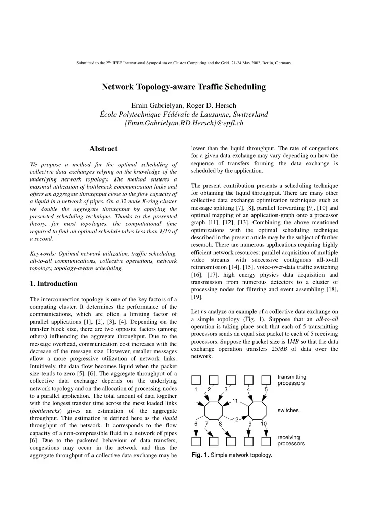
efficient network resources: parallel acquisition of multiple video streams with successive contiguous all-to-all retransmission [14], [15], voice-over-data traffic switching [16], [17], high energy physics data acquisition and transmission from numerous detectors to a cluster of processing nodes for filtering and event assembling [18], [19]. Let us analyze an example of a collective data exchange on a simple topology (Fig. 1). Suppose that an all-to-all

• peration is taking place such that each of 5 transmitting

processors sends an equal size packet to each of 5 receiving

• processors. Suppose the packet size is 1MB so that the data

exchange operation transfers 25MB of data over the network.

Submitted to the 2nd IEEE International Symposium on Cluster Computing and the Grid. 21-24 May 2002, Berlin, Germany

Network Topology-aware Traffic Scheduling

Emin Gabrielyan, Roger D. Hersch École Polytechnique Fédérale de Lausanne, Switzerland {Emin.Gabrielyan,RD.Hersch}@epfl.ch

• Fig. 1. Simple network topology.

switches transmitting receiving processors processors 1 2 3 4 5 6 7 8 9 10 11 12

During the collective data exchange, links 1 to 10 transfer 5MB of data each (Fig. 1). Links 11 and 12 are the bottlenecks and transfer 6MB each. Suppose that the throughput of a link is 100MB/s. Since links 11 and 12 are the bottleneck, the longest transfer of the collective data exchange lasts . Therefore the liquid throughput

• f

the global

• peration

is . Let us now propose a schedule for successive data transfers and analyze its throughput. Intuitively, a good schedule for an all-to-all exchange is a round-robin schedule where at each step each sender has a receiver shifted by one position. Let us now examine the round-robin schedule of an all-to-all data exchange on the network topology of figure 1. Figure 2 shows that logical steps 1, 2 and 5 can be processed in the timeframe of a single transfer. But logical steps 3 and 4 can not be processed in a single timeframe, since there are two transfers trying to simultaneously use the same links 11 and 12, causing a congestion. Two conflicting transfers need to be scheduled in two single timeframe substeps. Thus the round-robin schedule takes 7 timeframes instead of the expected 5 and accordingly, the throughput of the round- robin all-to-all exchange is: . It is therefore less than the liquid throughput (416.67MB/s). Can we propose an improved schedule for the all-to-all exchange such that the liquid throughput is reached? By ensuring that at each step the bottlenecks are always used, we create an improved schedule, having the performance of the network’s liquid throughput (Fig. 3). According to this improved schedule only 6 steps are needed for the implementation of the collective operation, i.e. the throughput is: . Section 2 shows how to describe the liquid throughput as a function of the number of contributing processing nodes and their underlying network topologies. An introduction to the formal theory of traffic scheduling is given in section 3. Section 4 presents measurements for the considered sub- topologies and draws the conclusions.

• 2. Throughput as a function of sub-topology

In order to evaluate the throughput of collective data exchanges we need to specify along an independent axis the number of processing nodes as well as significant variations of their underlying network topologies. To simplify the model let us limit the configuration to an identical number of receiving and transmitting processors forming successions of node pairs. The applications perform all-to-all data exchanges over the allocated nodes (each transmitting processor sends one packet to each receiving processor). Let us demonstrate how to create variations of processing node allocations by considering the specific network of the Swiss-T1 cluster (called henceforth T1, see Fig. 4). The network of the T1 forms a K-ring [20] and has a static 6MB 100MB s ⁄ ( ) ⁄ 0.06s = 25MB 0.06s ⁄ 416.67MB s ⁄ =

step 1 timeframe 1 step 3 timeframe 3 step 3 timeframe 4 step 4 timeframe 5 step 4 timeframe 6 step 5 timeframe 7 step 2 timeframe 2

• Fig. 2. Round-robin schedule of transfers.

25MB 7 1MB 100MB s ⁄

• ⎝

⎠ ⎛ ⎞ × ⎝ ⎠ ⎛ ⎞ ⁄ 357.14MB s ⁄ = 25MB 6 1MB 100MB s ⁄

• ⎝

⎠ ⎛ ⎞ × ⎝ ⎠ ⎛ ⎞ ⁄ 416.67MB s ⁄ =

• Fig. 3. An optimal schedule.

timeframe 1 timeframe 2 timeframe 3 timeframe 4 timeframe 5 timeframe 6

routing scheme. The throughputs of all links are identical and are equal to 86MB/s. The cluster consists of 64 processors paired into 32 nodes [21], [22]. Since the T1 cluster incorporates 32 nodes, there exist possible allocations of nodes to an

• application. Considering only the number of nodes in front
• f each switch, there are only

different processing node allocations, since there are 8 switches having each n used nodes ( ). Each allocation may be represented by a vector . With a model incorporating the given network topology and routing tables, we can compute the liquid throughput of an all-to-all traffic for any allocation. The full set of 390625 allocation vectors is given as input to the model and the liquid throughput is computed for each input vector. For the T1’s network, only 363 different values of liquid throughput are formed and thus the set of 390625 is partitioned into 363 different subsets. Each of the obtained 363 key sub-topologies is characterized by its liquid throughput and the number of allocated nodes (see Fig. 5). The figure demonstrates that depending on the sub- topology, the liquid throughput for a given number of nodes may considerably vary. For the purpose of enumerating the 363 sub-topologies we sort these sub-topologies according to the number of nodes and within the same number of nodes according to the value of the liquid throughput. Figure 6 demonstrates the liquid throughput of the network together with the throughput of an imaginary full crossbar network. The horizontal axis represents the collection of the 363 sub- topologies together with the number of contributing processing nodes (in parentheses).

• 3. Liquid schedules

This section proposes a formal model of a collective data

• exchange. In this model a single point-to-point transfer is

represented by the set of communication links forming the 232 4294967296 = 58 390625 = n 4 ≤ ≤ n0 n1 n2 n3 n4 n5 n6 n7

2 4 5 6

Network link Routing information

3 7 1 PR63 PR00 PR01 PR00 P R 2 PR04 PR06 P R 8 PR10 PR12 PR14 PR16 P R 1 8 PR20 PR22 P R 2 4 PR26 PR28 PR30 PR32 P R 3 4 PR36 PR38 P R 4 PR42 PR44 PR46 PR48 P R 5 PR52 PR54 P R 5 6 PR58 PR60 PR62 P R 6 1 PR59 PR57 P R 5 5 PR53 PR51 PR49 PR47 P R 4 5 PR43 PR41 P R 3 9 PR37 PR35 PR33 PR31 P R 2 9 PR27 PR25 P R 2 3 PR21 PR19 PR17 PR15 P R 1 3 PR11 PR09 P R 7 PR05 PR03 PR01

Sending Processor Receiving Processor Node

• Fig. 4. Architecture of the T1 cluster computer.

N00 N 1 N02 N03 N04 N05 N 6 N07 N08 N09 N10 N11 N12 N13 N 1 4 N15 N16 N17 N18 N19 N20 N21 N 2 2 N23 N24 N25 N26 N27 N28 N29 N30 N 3 1 N00

Switch

path between a transmitting and a receiving processor. The collective data exchange comprises a set of transfers having identical packet sizes. A sending processor may transfer a packet to a given receiving processor not more than once.

• DEFINITIONS. A transfer is a set of links (i.e. the path from

a sending processor to a receiving processor). A traffic is a set of transfers (see Fig. 7). A link l is utilized by a transfer x if . A link l is utilized by a traffic X if l is utilized by a transfer of X. Let a and b be transfers of a traffic X, the transfer b is in congestion with a, if b uses a link utilized by

• a. A sub-traffic of X (a subset of X) is simultaneous if it

forms a collection of non-congesting transfers. A simultaneous subset of a traffic is processed in the timeframe of a single transfer. The load of link l in the traffic X is the number of transfers in X using l. The duration

• f a traffic X is the maximal value of the

load among all links involved in the traffic. The links having maximal load values are called bottlenecks. The liquid throughput of a traffic X is the ratio multiplied by a single link throughput, where is the number of transfers in the traffic X. For example, the traffic X shown in figure 7 has a number of transfers and the duration of the traffic is . Therefore the aggregate liquid throughput is the ratio

• f a single

link throughput, i.e. , supposing a single link throughput of 100 MB/s. Recall that a partition of X is a disjoint collection of non- empty subsets of X whose union is X [23]. A schedule

• f

a traffic X is a collection of simultaneous subsets of X partitioning the traffic X. A timeframe of a schedule is an element of . The length

• f a schedule

is the number of timeframes in . A schedule of a traffic is

• ptimal if the traffic does not have any shorter schedule. If

the length of a schedule is equal to the duration of the traffic then the schedule is liquid. A liquid schedule is

• ptimal, but the inverse is not always true, meaning that a

traffic may not have a liquid schedule (the demonstration is beyond the scope of this article). Figure 8 shows a liquid schedule of the collective traffic shown in figure 7.

200 400 600 800 1000 1200 1400 1600 1800 4 8 12 16 20 24 28 32 Number of contributing nodes Liquid throughput (MB/s) U p p e r b

• u

n d L

• w

e r b

• u

n d

Fig 5. Liquid throughput in relation to the number

• f nodes with variations according to sub-

topologies.

l x ∈ Λ X ( ) # X ( ) Λ X ( ) ⁄ # X ( ) # X ( ) 25 = Λ X ( ) 6 = 25 6 ⁄ 25 6 ⁄ ( ) 100 × MB s ⁄ α α α # α ( ) α α

400 800 1200 1600 2000 2400 2800 ( ) 3 ( 9 ) 6 ( 1 1 ) 9 ( 1 2 ) 1 2 ( 1 4 ) 1 5 ( 1 5 ) 1 8 ( 1 6 ) 2 1 ( 1 8 ) 2 4 ( 1 9 ) 2 7 ( 2 ) 3 ( 2 2 ) 3 3 ( 2 4 ) 3 6 ( 3 ) Aggregate throughput (MB/s)

• Fig. 6. Liquid and crossbar throughputs on T1.

Crossbar throughput Liquid throughput {l1, l6}, {l1, l7}, {l1, l8}, {l1, l12, l9}, {l1, l12, l10}, {l2, l6}, {l2, l7}, {l2, l8}, {l2, l12, l9}, {l2, l12, l10}, {l3, l6}, {l3, l7}, {l3, l8}, {l3, l12, l9}, {l3, l12, l10}, {l4, l11, l6}, {l4, l11, l7}, {l4, l11, l8}, {l4, l9}, {l4, l10}, {l5, l11, l6}, {l5, l11, l7}, {l5, l11, l8}, {l5, l9}, {l5, l10}

• Fig. 7. All-to-all traffic.

} }

l1 l2 l3 l4 l5 l6 l7 l8 l9 l10 l11 l12

The duration of a traffic X is the load of its bottlenecks. Consider l as one of the bottlenecks of X. The load of l is the number of transfers in X using l. Now let be a schedule on X. By definition is a collection of simultaneous subsets of X, partitioning X. Since partitions X, a transfer of X (using l) shall be found in one and only one of the timeframes of . Since a timeframe of is simultaneous it may contain only one or no transfer using l. Therefore if the length of is equal to the number

• f transfers in X using the bottleneck l, then each timeframe
• f

shall contain a transfer using l. Inversely, if each timeframe of has a transfer using l, then the length of shall be equal to the number of transfers using l. Hence if a schedule is liquid then each of its timeframes uses all bottlenecks, and if all timeframes of a schedule use all bottlenecks then the schedule is liquid. In other words, we derived an equivalent condition for the liquidity of a schedule. The necessary and sufficient condition for the liquidity of a schedule is that all bottlenecks be used by each timeframe of the schedule. Let us define a simultaneous subset of X as a team of X if it uses all bottlenecks of X. Consequently, an equivalent condition for the liquidity of a schedule

• n X is that each

timeframe of be a team of X. Our goal is to design an algorithm that may partition a traffic so as to form a liquid schedule (whenever possible).

• DISCUSSION. Suppose A is a timeframe of a liquid schedule
• n a traffic X. Therefore A is a team of

. Remove the team A from X so as to form a new traffic . The duration of the new traffic is the load of the bottlenecks in . The bottlenecks of X are bottlenecks

• f

. The load of a bottleneck of X decreases by one in the new traffic . However the new traffic may have additional bottlenecks. The schedule without the element A is a schedule for with the previous length decreased by one. The new schedule has as many timeframes as the duration of the new traffic . Therefore is a liquid schedule on . In other words, if the traffic has a liquid schedule, then a schedule reduced by one team is a liquid schedule on the reduced traffic. This is the key point in searching for a liquid schedule. Consider traffic X as a problem whose solution is a liquid schedule . Assume a technique capable of generating the set of all teams of X. If X has a solution then a timeframe A of the schedule is a member of the set of all teams of X and is a schedule on . Therefore the problem X can be reduced into smaller problems. Examine each possible team A of X and search inductively (e.g. recursively) a solution for . If a solution exists for X, then the method will find it. If the method does not find a solution for X, and since we explored the full solution space, we conclude that X does not have a liquid schedule. We limit at each iteration our choice to the collection of

• nly those teams of the original traffic which are also teams
• f the current reduced sub-traffic. By doing so, we

considerably reduce the search space without affecting the solution space.

• DEFINITIONS. A simultaneous subset A of a traffic X is full

with respect to X if each transfer of is in congestion with a transfer of A. A team of X is called full team if it is a full simultaneous subset of X. We intend to limit the search space when building a liquid

• schedule. Let us modify a liquid schedule so as to convert
• ne of its teams into a full team. Let X (a traffic) have a

solution (a liquid schedule). Let A be a timeframe of . If A is not a full team of X, then, by moving the necessary transfers from other timeframes of , we can convert timeframe A to a full team. Evidently, the properties of liquidity (partitioning, simultaneousness and length) of will not be affected. Therefore if X has a solution then it has also a solution when one of its timeframes is full, hence the choice of the teams in the construction may be narrowed from the set of all teams to the set of full teams only. By a choice of a full team A of a traffic X we are faced with the new smaller problem of searching a liquid schedule for α α α α α α α α α {l1, l12, l9}, {l2, l7}, {l3, l8}, {l4, l11, l6}, {l5, l10} {l1, l12, l10}, {l2, l6}, {l4, l11, l7}, {l5, l9} {l1, l8}, {l2, l12, l9}, {l3, l6}, {l4, l10}, {l5, l11, l7} {l1, l7}, {l2, l8}, {l3, l12, l9}, {l5, l11, l6} {l1, l6}, {l2, l12, l10}, {l3, l7}, {l4, l11, l8} {l3, l12, l10}, {l4, l9}, {l5, l11, l8}

{

} } }

}

}

{ { {

{

} {

{

}

, , , , ,

• Fig. 8. A liquid schedule of the collective traffic shown in figure 7 (see also figure 3).

α α α α X A – X A – X A – X A – X A – X A – α X A – α A { } – X A – α A { } – X A – α α α α A { } – X A – X A – X A – α α α α

a traffic . The traffic may not have a solution,

• r it may not have even a team. In these cases we have to

backtrack to evaluate other choices. Evaluation of all choices ultimately leads to a solution if it exists. Figure 8 shows a liquid schedule built as explained above. Let us denote the timeframes in figure 8 as follows: , according to the order given in figure 8. Traffic X is the union of the timeframes . The schedule is constructed such that at any step i, the timeframe is a full team of the sub-traffic . The timeframe being a team of the sub- traffic incorporates therefore all bottlenecks of this sub-traffic (shown in bold). In order to be able to explore the full solution space for

• btaining a liquid schedule, we need to successively build

all full teams. We designed a procedure capable of generating (without repetitions) all successive full teams for an arbitrary traffic. It first builds skeletons, an intermediate collection of teams from a sub-traffic including only those transfers which comprise bottlenecks. Then it extends each skeleton by applying variations of all non-congesting transfers in order to build up all full teams.

• 5. Results and conclusion

For an unknown network topology only two intuitively reasonable schedules make sense, the round-robin and the random schedule. Measurements of the round-robin schedule and of the random schedule show a similar

• throughput. The round-robin schedule on a T1 cluster is

shown in figure 9. The amount of data transferred from one processor to another processor is equal to 2MB and the transfer block size is 520KB. The figure presents the result

• f 4344 measurements of all-to-all data exchanges. For

each topology, 20 measurements were performed. The median of the collected results is represented as a small black square. The thick curve represents the liquid

• throughput. The thin curve below the graph of the liquid

throughput represents the theoretically predicted throughput of the round-robin schedule, computed for the model of the T1 cluster. The measured throughput is higher than the predicted

• throughput. This increase in throughput in the real network

is explained by a “semifluid” behaviour of transfers: time shifts in packet transfers tend to reduce congestions. Nevertheless the measured round-robin throughput for a large number of sub-topologies is only 50% of the liquid throughput. X A – X A – A1 A2 A3 A4 A5 A6 , , , , , { } X Ai

i 1 = 6

∪

= Ai X Ak

k 1 = i 1 –

∪

– Ai X Ak

k 1 = i 1 –

∪

–

200 400 600 800 1000 1200 1400 1600 1800 2000 6 8 9 9 1 1 1 1 1 1 2 1 2 1 2 1 3 1 3 1 4 1 4 1 4 1 5 1 5 1 5 1 6 1 6 1 7 1 7 1 7 1 8 1 8 1 9 1 9 1 9 2 2 2 1 2 1 2 2 2 2 2 3 2 4 2 5 2 6 2 7 3 Number of contributing nodes for the 363 sub-topologies All-to-all throughput (MB/s)

• Fig. 10. Predicted liquid throughput and measured throughput according to the computed liquid schedule.

measurements on T1 according to the computed liquid schedule liquid throughput 200 400 600 800 1000 1200 1400 1600 1800 9 11 13 14 15 16 18 19 21 23 26 Numbers of nodes for the 363 sub-topologies Aggregate throughput (MB/s)

• Fig. 9. Throughput of the round-robin schedule.

measured round-robin liquid throughput predicted round-robin T1 Cluster

Thanks to the presented theory, we strongly reduce the search space of liquid schedules. The computation time of a liquid schedule takes for more than 97% of the considered sub-topologies of the T1 cluster less than 1/10 of a second

• n a single 500MHz Alpha processor. Figure 10 shows the

measured aggregate throughput of an all-to-all collective traffic executed on T1, optimized by applying our liquid schedule based traffic partitioning technique. Each black dot represents the median of 7 measurements. The horizontal axis represents the 363 sub-topologies as well as the number of contributing nodes. Processor to processor transfers have a size of 5MB, transferred as a single message of 5MB. The measured all-to-all aggregate throughputs (black dots) are close to the theoretically computed liquid throughput (gray line). For many sub- topologies, the proposed liquid scheduling technique allows to increase the aggregate throughput by at least a factor of two compared with a simple round-robin or random schedule.

References

[1]

• H. Sayoud, K. Takahashi, B. Vaillant, “Designing communi-

cation network topologies using steady-state genetic algo- rithms”, IEEE Communications Letters, Vol. 5, No. 3, March 2001, 113-115. [2] Pangfeng Liu, Jan-Jan Wu, Yi-Fang Lin, Shih-Hsien Yeh, “A simple incremental network topology for wormhole switch-based networks”, Proc. 15th International Parallel and Distributed Processing Symposium, 2001, 6-12. [3] P.K.K. Loh, Wen Jing Hsu, Cai Wentong, N. Sriskanthan, “How network topology affects dynamic loading balanc- ing”, IEEE Parallel & Distributed Technology: Systems & Applications, Vol. 4, No. 3, 25-35. [4]

• V. Puente, C. Izu, J. A. Gregorio, R. Beivide, J. M. Prellezo,
• F. Vallejo, “Improving parallel system performance by

changing the arrangement of the network links”, Proc. of the International Conference on Supercomputing, May 2000, 44-53. [5]

• M. Naghshineh, R. Guerin, “Fixed versus variable packet

sizes in fast packet-switched networks”, Proc.Twelfth Annual Joint Conference of the IEEE Computer and Com- munications Societies INFOCOM '93., Networking: Foun- dation for the Future, IEEE Press, Vol. 1, 1993, 217-226. [6] Benjamin Melamed, Khosrow Sohraby, Yorai Wardi, “Mea- surement-Based Hybrid Fluid-Flow Models for Fast Multi- Scale Simulation”, DARPA/NMS BAA 00-18 AGREE- MENT No. F30602-00-2-0556, http://www.darpa.mil/ito/ research/nms/meetings/nms2001apr/Rutgers-SD.pdf [7] K.G. Yocum, J.S. Chase, A.J. Gallatin, A.R. Lebeck, “Cut- through delivery in Trapeze: An Exercise in Low-Latency Messaging”, 6th IEEE International Symposium on High Performance Distributed Computing, 1997, 243-252. [8] N.M.A. Ayad, F.A. Mohamed, “Performance analysis of a cut-through vs. packet-switching techniques”, Proc. Second IEEE Symposium on Computers and Communications, 1997, 230-234. [9] Thilo Kielmann, Henri E. Bal, Sergei Gorlatch, Kees Ver- stoep, Rutger F.H. Hofman, “Network Performance-aware Collective Communication for Clustered Wide Area Sys- tems”, Parallel Computing, Vol. 27, No. 11, 2001, 1431- 1456. [10] Il Kyu Park, Youngseok Lee, Yanghee Choi, “Stable load control with load prediction in multipath packet forward- ing”, Proc. 15th International Conference on Information Networking, 2001, 437-444. [11] Sibabrata Ray, Hong Jiang, Jitender S. Deogun, “A parallel algorithm for mapping a special class of task graphs onto linear array multiprocessors”, Proc. of the ACM Sympo- sium on Applied Computing, April 1994, 473-477. [12] Y. Xie, W. Wolf, “Allocation and scheduling of conditional task graph in hardware/software co-synthesis”, Proc. of the

• Conf. on Design, Automation and Test in Europe (DATE

2001) March 2001, 620-625. [13] Chiang Chuanwen, Lee Chungnan, Chang Mingjyh, “A dynamic grouping scheduling for heterogeneous Internet- centric metacomputing system”, Proc. 8th International Conference on Parallel and Distributed Systems, ICPADS 2001, 77 -82. [14] S.-H.G. Chan, “Operation and cost optimization of a distrib- uted servers architecture for on-demand video services”, IEEE Communications Letters, Vol. 5, No. 9, Sept. 2001, 384-386. [15] Dinkar Sitaram, Asit Dan, Multimedia Servers, Morgan Kaufmann Publishers, San Francisco California, ISBN 1- 55860-430-8, 2000, 69-73. [16] H.323 Standards, http://www.openh323.org/standards.html [17] D.A. Fritz, D.W. Moy, R.A. Nichols, “Modeling and simula- tion of Advanced EHF efficiency enhancements”, Proc. of Military Communications Conference, IEEE MILCOM 1999, Vol. 1, 354-358. [18] ATLAS Collaboration, CERN, Technical Progress Report, http://press.web.cern.ch/Atlas/GROUPS/DAQTRIG/TPR/ PDF_FILES/TPR.bk.pdf [19] Large Hadron Collider, Computer Grid project, CERN, 20.09.2001, http://press.web.cern.ch/Press/Releases01/ PR10.01EGoaheadGrid.html [20] P. Kuonen, “The K-Ring: a versatile model for the design of MIMD computer topology”, Proc. of the High-Performance Computing Conference (HPC'99), San Diego, USA, April 1999, 381-385. [21] Pierre Kuonen, Ralf Gruber, “Parallel computer architec- tures for commodity computing and the Swiss-T1 machine”, EPFL Supercomputing Review, Nov 99, pp. 3-11, http:// sawww.epfl.ch/SIC/SA/publications/SCR99/scr11- page3.html [22] Ralf Gruber, “Commodity computing results from the Swiss-Tx project Swiss-Tx Team”, http://www.grid-comput- ing.net/documents/Commodity_computing.pdf [23] Paul R. Halmos, Naive Set Theory, Springer-Verlag New York Inc, ISBN 0-387-90092-6, 1974, 26-29.