Network Flow IV - Given information about flights that an airline - PowerPoint PPT Presentation

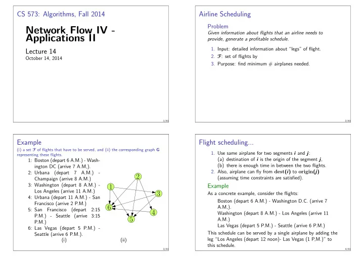
CS 573: Algorithms, Fall 2014 Airline Scheduling Problem Network Flow IV - Given information about flights that an airline needs to Applications II provide, generate a profitable schedule. 1. Input: detailed information about “legs” of flight. Lecture 14 2. F : set of flights by October 14, 2014 3. Purpose: find minimum # airplanes needed. 1/61 2/61 Example Flight scheduling... (i) a set F of flights that have to be served, and (ii) the corresponding graph G 1. Use same airplane for two segments i and j : representing these flights. (a) destination of i is the origin of the segment j , 1: Boston (depart 6 A.M.) - Wash- (b) there is enough time in between the two flights. ington DC (arrive 7 A.M,). 2. Also, airplane can fly from dest ( i ) to origin ( j ) 2: Urbana (depart 7 A.M.) - 2 (assuming time constraints are satisfied). Champaign (arrive 8 A.M.) 3: Washington (depart 8 A.M.) - Example 1 Los Angeles (arrive 11 A.M.) 3 As a concrete example, consider the flights: 4: Urbana (depart 11 A.M.) - San Boston (depart 6 A.M.) - Washington D.C. (arrive 7 Francisco (arrive 2 P.M.) 6 A.M,). 5: San Francisco (depart 2:15 4 Washington (depart 8 A.M.) - Los Angeles (arrive 11 P.M.) - Seattle (arrive 3:15 5 A.M.) P.M.) Las Vegas (depart 5 P.M.) - Seattle (arrive 6 P.M.) 6: Las Vegas (depart 5 P.M.) - This schedule can be served by a single airplane by adding the Seattle (arrive 6 P.M.). leg “Los Angeles (depart 12 noon)- Las Vegas (1 P,M.)” to (i) (ii) this schedule. 3/61 4/61

Modeling the problem Solution 1. Reduction to computation of circulation. 1. model the feasibility constraints by a graph. 2. Build graph H . 2. G : directed graph over flight legs. 3. ∀ leg i , two new vertices u i , v i ∈ VH . 3. For i and j (legs), ( i → j ) ∈ E(G) ⇐ ⇒ same airplane s : source vertex. t : sink vertex. can serve both i and j . 4. Set demand at t to k , Demand at s to be − k . 4. G is acyclic. 5. Flight must be served: New edge e i = ( u i → v i ) , for leg i . 5. Q: Can required legs can be served using only k airplanes? Also ℓ ( e i ) = 1 and c ( e i ) = 1 . 6. If same plane can so i and j (i.e., ( i → j ) ∈ E(G) ) then add edge ( v i → u j ) with capacity 1 to H . 7. Since any airplane can start the day with flight i : add an edge ( s → u i ) with capacity 1 to H , ∀ i . 8. Add edge ( v j → t ) with capacity 1 to G , ∀ j . 9. Overflow airplanes: “overflow” edge ( s → t ) with capacity k . Let H denote the resulting graph. 5/61 6/61 Example of resulting graph Lemma The resulting graph H for the instance of airline scheduling show before. Lemma k ∃ way perform all flights of F ≤ k planes ⇐ ⇒ ∃ circulation 1 , 1 in H . u 1 v 1 Proof. 1 , 1 u 2 v 2 1. Given feasible solution → translate into valid circulation. 1 , 1 u 3 v 3 2. Given feasible circulation... − k k 3. ... extract paths from flow. 1 , 1 s t u 4 v 4 4. ... every path is a plane. 2 1 , 1 u 5 v 5 1 3 1 , 1 u 6 v 6 6 4 5 7/61 8/61

Extensions and limitations 1. a lot of other considerations: (i) airplanes have to undergo long term maintenance treatments every once in awhile, Part I (ii) one needs to allocate crew to these flights, (iii) schedule differ between days, and (iv) ultimately we interested in maximizing revenue. Image Segmentation 2. Network flow is used in practice, real world problems are complicated, and network flow can capture only a few aspects. 3. ... a good starting point. 9/61 10/61 Image Segmentation What is the input... 1. Input is a bitmap on a grid. Input is an image. 2. Every grid node represents a Partition image into background and foreground. pixel 3. Convert grid into a directed graph G , 4. Input: (i) N × N bitmap. G = (V , E) . (ii) ∀ pixel i : foreground value (i) (ii) f i ≥ 0 . The (i) input image, and (ii) a possible segmentation of the (iii) ∀ pixel i : background image. value b i . (iv) ∀ i , j adjacent: separation penalty p ij . (we assume that p ij = p ji ) 11/61 12/61

Problem statement Restating problem... Maximizing: Problem   Given input as above, partition V (the set of pixels) into two � � � �  . disjoint subsets F and B , such that q ( F , B ) = ( f i + b i ) − f i + b j + p ij i ∈ v i ∈ B j ∈ F � � � ( i , j ) ∈ E , | F ∩{ i , j }| =1 q ( F , B ) = f i + b i − p ij . Equivalent to minimizing u ( F , B ) : i ∈ F i ∈ B ( i , j ) ∈ E , | F ∩{ i , j }| =1 � � � is maximized. u ( F , B ) = f i + b j + p ij . (1) i ∈ B j ∈ F Rewrite q ( F , B ) as: ( i , j ) ∈ E , | F ∩{ i , j }| =1 � � � q ( F , B ) = f i + b j − p ij i ∈ F j ∈ B ( i , j ) ∈ E , | F ∩{ i , j }| =1   � � � �  . = ( f i + b i ) − f i + b j + p ij i ∈ v i ∈ B j ∈ F ( i , j ) ∈ E , | F ∩{ i , j }| =1 13/61 14/61 Solution continued... Solution continued... b i i 1. Compute a minimum cut in a graph. Price = u ( F , B ) . f i s t f i b i s i f j j 2. A toy example: t b j 1. Two pixel bitmap: 3. two possible cuts in the graph: 2. Captures background/foreground prices. But... ignores (i) ( { s , i } , { t } ) : price b i . separation penalties... (ii) ( { s } , { i , t } ) : price f i . b i f i i 4. Every len 2 path s � t forces mincut to choose one of s p ij p ij t f j j edges. b j 3. Mincut “prefers” the edge with lower price. 4. Price of cut in graph is corresponding value of u ( F , B ) . 5. mincut-cut in the resulting graph would corresponds to the required segmentation. 15/61 16/61

Recap... Solution continues... By the above discussion: 1. Given directed grid graph G = (V , E) . Lemma 2. s , y : add two special source and sink vertices. A minimum cut ( F , B ) in H minimizes u ( F , B ) . 3. ∀ i ∈ V ,: add edge e i = ( s → i ) . Using the minimum-cut max-flow theorem, we have: c ( e i ) = f i . 4. Add e ′ i = ( j → t ) with capacity c ( e ′ Theorem i ) = b i . One can solve the segmentation problem, in polynomial time, 5. ∀ i . j adjacent: by computing the max flow in the graph H . assign the capacity p ij to the edges ( i → j ) and ( j → i ) H : resulting graph. 17/61 18/61 Project Selection 1. company which can carry out some projects. 2. P : set of possible projects. Part II 3. ∀ i ∈ P : a revenue p i . 4. p i > 0 is a profitable project and p i < 0 is a losing project. Projection selection 5. There is dependency between projects. 6. G = ( P , E ) : ( i → j ) ∈ E ⇐ ⇒ j is a prerequisite for i . 19/61 20/61

Definition Project selection example Definition ∞ − 2 − 3 − 5 − 8 A set X ⊂ P is feasible if for all i ∈ X , all the prerequisites of i are also in X . Formally, for all i ∈ X , with an edge ( i → j ) ∈ E , we have j ∈ X . ∞ The profit associated with a set of projects X ⊆ P is ∞ ∞ ∞ profit ( X ) = � i ∈ X p i . 4 6 2 3 Problem - Project Selection Problem ∞ ∞ Select a feasible set of projects maximizing the overall profit. 21/61 22/61 The reduction Example: Resulting network 1. Use mincut again. t 2. Add s and t to G . 2 8 3 3. Perform the following modifications: 5 60 4. ∀ i ∈ P with p i > 0 : add edge e i = ( s → i ) . − 2 − 3 − 5 − 8 with c ( e i ) = p i . 60 5. ∀ j ∈ P with p j < 0 : add edge e ′ j = ( j → t ) . 60 60 60 Set c ( e ′ j ) = − p j . 4 � 6 2 3 60 60 6. C = i ∈ P , p i > 0 p i : upper bound on profit. 7. Set capacity of all original (dependency) edges in G to 2 6 3 4 C . 4 s Let H denote the resulting network. 23/61 24/61

Solution continued Lemma Lemma 1. X ⊆ P : Set of feasible projects. c ( X ′ , Y ′ ) = C − � 2. X ′ = X ∪ { s } and Y ′ = ( P \ X ) ∪ { t } . i ∈ X p i = C − profit ( X ) . 3. Consider the s - t cut ( X ′ , Y ′ ) in H . Proof 4. No E(G) is in ( X ′ , Y ′ ) since X is a feasible set. 1. The edges of H are either: (i) original edges of G , (ii) emanating from s , and (iii) edges entering t . 2. X feasible = ⇒ no edges of type (i) in cut. 3. Edges entering t contribute: � β = − p i . i ∈ X and p i < 0 25/61 26/61 Proof continued Lemma Proof. Lemma If ( X ′ , Y ′ ) is a cut with capacity at most C in G , then the set Edges leaving s contribute: X = X ′ \ { s } is a feasible set of projects. � � � γ = p i = p i − p i Namely, cuts ( X ′ , Y ′ ) of capacity ≤ C in H corresponds i ∈ P , p i > 0 i ∈ X and p i > 0 i / ∈ X and p i > 0 one-to-one to feasible sets which are profitable. � = C − p i , Proof. i ∈ X and p i > 0 Since c ( X ′ , Y ′ ) ≤ C it must not cut any of the edges of G , by the definition of C . The capacity of the cut ( X ′ , Y ′ ) is since the price of such an edge is 4 C . As such, X must be a feasible set.   � �  C −  β + γ = ( − p i ) + p i i ∈ X and p i < 0 i ∈ X and p i > 0 � = C − p i = C − profit ( X ) , i ∈ X 27/61 28/61