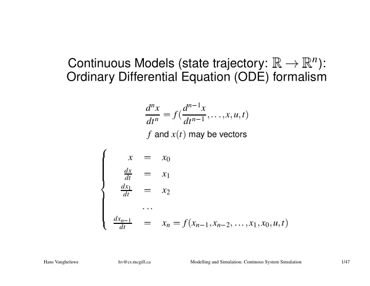
n ): Continuous Models (state trajectory: Ordinary Differential - PowerPoint PPT Presentation

✠ ✞ ✝ ✞ ✞ ✞ ✞ ✞ ✞ ✞ ✞ ✟ ✞ ✞ � ✞ ✞ ✞ ✞ ✞ � � ✡ ☎ ☎ � � ✆ ✁ ✁ ✆ ✄ ✄ � ✄ ✁ ✄ ✂ ☎ ☎ ✂ ☎ ✄ ☎ ☎ ☎ ✄ ✄ ✄ ✂ ✄ ✄ ✆ ✂ ☎ n ): Continuous Models (state trajectory: Ordinary Differential Equation (ODE) formalism d n x d n 1 x f x u t dt n dt n 1 f and x t may be vectors x x 0 dx x 1 dt dx 1 x 2 dt dx n 1 x n f x n x n x 1 x 0 u t 1 2 dt Hans Vangheluwe hv@cs.mcgill.ca Modelling and Simulation: Continous System Simulation 1/47

✆ ✁ ✁ ✆ � ✎ � ✎ ✆ ✆ ✁ ☞ ✆ ✄ ✁ ✁ ☛ ✁ ☞ ✄ ✁ ✆ � ✄ ✁ ✆ ✄ ✄ ✁ ✄ ✆ ☛ ✆ ✁ ✁ ☞ ✆ Euler discretisation dx f x u t dt ∆ t x t i x t i ✆✍✌ f x t i u t i t i ∆ t ∆ t ∆ t f x t i x t i x t i u t i t i Hans Vangheluwe hv@cs.mcgill.ca Modelling and Simulation: Continous System Simulation 2/47

� ☎ ✎ � ✁ ☞ ✏ ✏ ✑ ☞ ✌ ☞ ✏ ✆ ☎ ✁ ☎ � ✆ ✆ ☞ ✑ ✁ ☞ Taylor Series Expansion ∆ t 2 d 2 x ∆ t 3 d 3 x ∆ t dx ∆ t x t i x t i t i t i t i dt 2 dt 3 1! dt 2! 3! Is EXACT if expansion is not truncated ∆ t N 1 ERROR O if truncated after term N Beyond first derivative, use difference formulas ERROR ε N approx N approx N 1 Hans Vangheluwe hv@cs.mcgill.ca Modelling and Simulation: Continous System Simulation 3/47

✆ � ✑ ✒ � ☞ ✁ ✄ ✄ Integration Methods: Euler Single-step α 0 x 0 ∆ t f x i x i t i x i i 0 1 Unsymmetrical: uses only derivative in begin point. Hans Vangheluwe hv@cs.mcgill.ca Modelling and Simulation: Continous System Simulation 4/47

☞ � ✄ � ✆ ✆ ✑ ✄ ✁ ☞ ☞ � ☞ ✄ � ✒ ✁ Integration Methods: Modified Euler Single-step α 0 x 0 ∆ t f k 1 t i x i ∆ t f ∆ t k 2 t i x i k 1 k 1 k 2 x i x i i 0 1 2 2 Symmetrical: uses derivative in begin and end point. Hans Vangheluwe hv@cs.mcgill.ca Modelling and Simulation: Continous System Simulation 5/47

✄ ✁ ✒ � ✄ ☞ � � ✁ ✑ ✄ ✆ ✆ ☞ � ☞ Integration Methods: Midpoint Single-step α 0 x 0 ∆ t f k 1 t i x i k 1 ∆ t ∆ t f k 2 t i x i 2 2 0 x i x i k 2 i 1 Symmetrical: halfway point. Hans Vangheluwe hv@cs.mcgill.ca Modelling and Simulation: Continous System Simulation 6/47

☞ � ✄ � ✆ ✆ ✑ ✄ ✁ ☞ ☞ � ☞ ✄ � ✒ ✁ Integration Methods: Heun Single-step α 0 x 0 ∆ t f k 1 t i x i 2 k 1 2 ∆ t ∆ t f k 2 t i x i 3 3 k 1 3 k 2 x i x i i 0 1 4 4 Hans Vangheluwe hv@cs.mcgill.ca Modelling and Simulation: Continous System Simulation 7/47

✆ ✄ ✆ � ✄ ✁ ✁ � ✆ ☞ ✄ ✓ ✁ ☞ ☞ ✂ � ✄ ✑ ✓ � Integration Methods: Runge-Kutta Methods Single-step, q stages (function evaluations per step) ∆ t φ x i ; ∆ t x i x i t i 1 q ∑ φ x i ; ∆ t ω i k i t i i 1 Explicit method: i 1 ∑ ∆ t α i ∆ t β ij k j α 1 0 k i f t i x i j 1 Hans Vangheluwe hv@cs.mcgill.ca Modelling and Simulation: Continous System Simulation 8/47

✄ ✓ � ✆ ✁ ✁ ☞ ✄ ✄ ✕ ☞ ✔ ✔ ✆ Implicit method: q ∑ ∆ t α i ∆ t β ij k j k i f t i x i j 1 nonlinear set of equations in k i explicit is a special case Order p : exact solution up to polynomial of order p can determine α i ω i β ij For explicit method of order p , at least q min p stages are required: p 1 2 3 4 5 6 7 ... q_min(p) 1 2 3 4 6 7 9 ... Hans Vangheluwe hv@cs.mcgill.ca Modelling and Simulation: Continous System Simulation 9/47

� ✁ ✄ � ✑ ✆ ☞ ✆ ☞ ✒ ✄ � ✄ ☞ ✁ ☞ ☞ � ☞ ✆ ☞ ✄ ✄ ✁ ☞ � ☞ ☞ � ✆ ✁ Integration Methods: Runge-Kutta 4 Single-step α 0 x 0 ∆ t f k 1 t i x i k 1 ∆ t ∆ t f k 2 t i x i 2 2 k 2 ∆ t ∆ t f k 3 t i x i 2 2 ∆ t f ∆ t k 4 t i x i k 3 k 1 k 2 k 3 k 4 x i x i i 0 1 6 3 3 6 Hans Vangheluwe hv@cs.mcgill.ca Modelling and Simulation: Continous System Simulation 10/47

� ✁ ✂ ✁ ✄ ✁ ✁ ✂ ✄ ✄ ☞ ✂ � ✆ ✄ ✑ ✒ ✄ ✁ � ✄ ✒ ✄ � ✆ ✆ � ✂ ✑ ✑ ✂ � ✁ ☞ ☞ ✆ ✁ � Integration Methods: Adams-Bashforth Multi-step: need lower-step methods for start-up 2-step α 0 x 0 α 1 x 1 ∆ t x i x i 3 f t i x i f t i x i i 1 1 1 1 ✆✍✌ 2 3-step α 0 x 0 α 1 x 1 α 2 x 2 ∆ t x i x i 23 f t i x i 16 f t i x i 5 f t i x i i 2 1 1 1 2 2 ✆✍✌ 12 Hans Vangheluwe hv@cs.mcgill.ca Modelling and Simulation: Continous System Simulation 11/47

✁ ✆ ✄ ✄ ✁ ✂ ✆ ✄ ✑ ✆ ✁ ☞ ✂ ✁ ✄ ✂ ✂ ✄ ✂ ✁ ✒ ✑ � ☞ � � � � 4-step α 0 x 0 α 1 x 1 α 2 x 2 α 3 x 3 x i 1 ∆ t x i 55 f t i x i 59 f t i x i 37 f t i x i 9 f t i x i i 3 1 1 2 2 3 3 ✆✍✌ ✆✍✌ 24 Hans Vangheluwe hv@cs.mcgill.ca Modelling and Simulation: Continous System Simulation 12/47

✖ ✁ ☞ ✆ ✑ ✁ ✗ ✂ ✖ ✄ ✄ ✂ ✑ ✆ ☞ ✁ ✁ ✁ ✂ ☞ ✄ ✂ ✂ � ✆ ✆ ✄ ✑ ✒ ✗ ✄ ✁ ✑ ✄ ✔ ☎ ☎ � ☎ ✄ � ✄ � � ✄ ✒ � ✆ ✄ ✖ ✆ ✗ ✂ ✑ ✄ � ✂ ✂ ✁ ☞ ☞ ✆ ✁ ✔ Integration Methods: Milne Predictor-corrector Predictor α 0 x 0 α 1 x 1 α 2 x 2 α 3 x 3 0 4 ∆ t 2 f 2 f 3 x x i t i x i f t i x i t i x i i 3 1 1 2 2 i 1 ✆✍✌ 3 Corrector k 1 k ∆ t 4 f x x i f t i x t i x i f t i x i 1 1 1 1 1 1 i 3 i i 2 k 1 2 Hans Vangheluwe hv@cs.mcgill.ca Modelling and Simulation: Continous System Simulation 13/47

� ✎ ✌ ✔ ✑ ✔ Adaptive Step-size Control want to attain pre-set minimum (step-wise) accuracy want mimimum computation Solution: use accuracy estimate to adjust (double/halve) step-size Obtaining accuracy estimate: 1. step halving ( e.g., RK4) 2. ε N approx N approx N 1 Hans Vangheluwe hv@cs.mcgill.ca Modelling and Simulation: Continous System Simulation 14/47

☞ ✑ ☞ ☞ � ☞ � ☞ ✙ ✙ ✙ ☞ ✁ ✆ ✓ ✆ ✑ � ✑ ☞ ✁ ☞ ✚ ☞ ✙ ✙ ✙ ☞ ✌ ☞ ✚ ✄ ☞ ✆ ✁ ✘ ✆ ✚ � � ✁ ☞ ✄ ✙ ✆ ✙ � ✙ ☞ ✚ ☞ ✑ ✄ ✚ ☞ ✌ ✆ ✙ ✙ ✙ ☞ � ✚ ✁ ✁ Adaptive Step-size Control RK4 + RK5 Runge-Kutta Fehlberg (embedded) ∆ t f k 1 t i x i ∆ t f a 2 ∆ t k 2 t i x i b 12 k 1 ∆ t f a 6 ∆ t k 6 t i x i b 61 k 1 b 62 k 2 b 65 k 5 ∆ t 6 x i x i c 1 k 1 c 2 k 2 c 6 k 6 O 1 ∆ t 5 x x i c 1 k 1 c 2 k 2 c 6 k 6 O i 1 ∑ 6 ε estim x i x c i c k i 1 i 1 i 1 i Hans Vangheluwe hv@cs.mcgill.ca Modelling and Simulation: Continous System Simulation 15/47

start set parameter set set initial set integrator values [ t_init, t_final] conditions set initial delta_t set integrator parameters t := t_init YES end t >= t_final ? NO estimate integration error E E<E_min E>E_max ? delta_t := delta_t*2 delta_t := delta_t/2 E in [E_min, E_max] integrate over [t, t_new] YES zero crossing NO occurred in [t,t_new] zero crossing ? t := t_new location t_zc t := t_zc iterate to consistent initial conditions Hans Vangheluwe hv@cs.mcgill.ca Modelling and Simulation: Continous System Simulation 16/47

✌ ✁ ✌ � ✆ ☞ ✁ � ✄ ✂ � ✆ ✌ ✂ � � ✌ ✌ ✌ � ✛ ✂ ☞ ☞ ✂ � ✛ � Stiff Systems u 998 u 1998 v v 999 u 1999 v u 0 1 v 0 0 u 2 y z v y z t 1000 t u 2 e e t 1000 t v e e Hans Vangheluwe hv@cs.mcgill.ca Modelling and Simulation: Continous System Simulation 17/47

☞ ☞ ✁ � ✑ ✑ ✛ ✔ ✛ � ✑ ✌ � ✑ ✑ � ✔ ✑ ✌ � ✛ ✆ Stiff Systems: solvers x cx ∆ tx Explicit: Forward Euler : x i x i 1 i c ∆ t x i 1 x i 1 ∆ tx Implicit: Backward Euler : x i x i 1 i 1 x i x i 1 1 c ∆ t Rosenbrock, Gear, . . . methods Hans Vangheluwe hv@cs.mcgill.ca Modelling and Simulation: Continous System Simulation 18/47

✄ � ☎ ☎ ☎ ✄ ✆ ✂ ✁ ✄ ✂ ✄ ✄ ✆ � ✁ ✄ Differential Algebraic Equations (DAE) d n x d n 1 x f x u t 0 dt n dt n 1 g x t 0 Residual Solvers DASSL (Petzold) http://www.engineering.ucsb.edu/ cse/software.html Hans Vangheluwe hv@cs.mcgill.ca Modelling and Simulation: Continous System Simulation 19/47

Causal continuous-time models Hans Vangheluwe hv@cs.mcgill.ca Modelling and Simulation: Continous System Simulation 20/47

Problems with algebraic model solving DAE-set != DAE-sequence No Yes cycles ? Set Sequence Set Sequence solve a = d - c sorting d = 2 a = b + 3 a = 3 b = c + a - 3 e = 3 b = a / 2 b = 3 c = 6 + d * e c = 6 + d * e d = 2 a = d - c e = 3 b = c + a - 3 linear nonlinear a = 0 b = 0 c = 6 d = 2 e = 3 Hans Vangheluwe hv@cs.mcgill.ca Modelling and Simulation: Continous System Simulation 21/47

Dependency Graph d e a = d - c b = c + a - 3 c = 6 + d * e c a d = 2 e = 3 b Hans Vangheluwe hv@cs.mcgill.ca Modelling and Simulation: Continous System Simulation 22/47