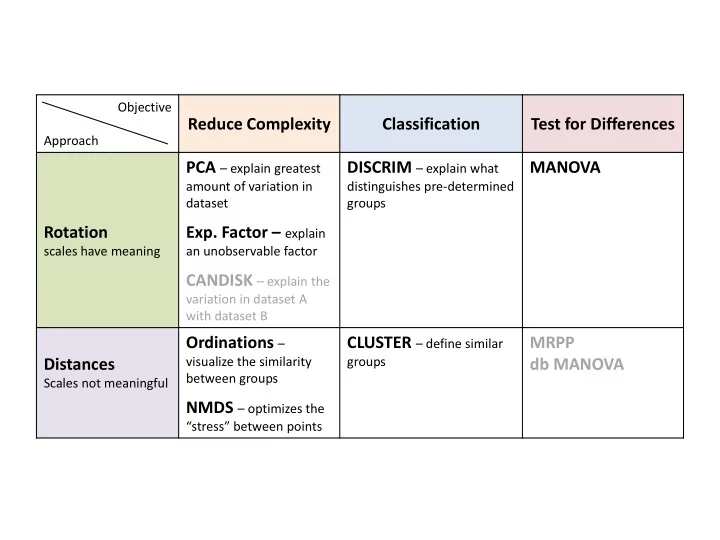
Multivariate Statistics Fundamentals Part 2: Distance-based - - PowerPoint PPT Presentation

Objective Approach

Reduce Complexity Classification Test for Differences Rotation

scales have meaning

PCA – explain greatest

amount of variation in dataset

• Exp. Factor – explain

an unobservable factor

CANDISK – explain the

variation in dataset A with dataset B

DISCRIM – explain what

distinguishes pre-determined groups

MANOVA Distances

Scales not meaningful

Ordinations –

visualize the similarity between groups

NMDS – optimizes the

“stress” between points

CLUSTER – define similar

groups

MRPP db MANOVA

Objective Approach

Reduce Complexity Classification Test for Differences Rotation

scales have meaning

PCA – explain greatest

amount of variation in dataset

• Exp. Factor – explain

an unobservable factor

CANDISK – explain the

variation in dataset A with dataset B

DISCRIM – explain what

distinguishes pre-determined groups

MANOVA Distances

Scales not meaningful

Ordinations –

visualize the similarity between groups

NMDS – optimizes the

“stress” between points

CLUSTER – define similar

groups

MRPP db MANOVA Today

Multivariate Statistics Fundamentals Part 2:

Distance-based Techniques

We use “Distance” to infer about similarity between data points Consider a 3D (3 variables) space:

Distance-based techniques

The green points are similar because they plot

• ut close together

The red points are also similar but this distance between them is larger than the green points We can use distances to determine if the grey point more similar to red or green group? Or is grey it’s own group?

Variable 3 Variable 1

Distance-based techniques

In General: If two points are closer together the distance is smaller – meaning variables are similar among points If two points are further apart the distance is greater – meaning variables are different among points Unlike rotation based techniques, distance-based techniques do not keep track of

• riginal scales

Data gets converted to represent similarity Data therefore becomes scale-less

The math behind distance-based techniques

x1 x2 y1 y2

A B C

It’s as simple as calculating the distance between points Simplest method is to calculate the Euclidian distance: Formula: C = 𝐵2 + 𝐶2 2D: 𝑒𝐹 = 𝑦1 − 𝑦2 2 + 𝑧1 − 𝑧2 2 Multi: 𝑒𝐹 = 𝑦1 − 𝑦2 2 + 𝑧1 − 𝑧2 2 + ⋯ + 𝑨1 − 𝑨2 2 We end up changing our data table:

Data.ID Varable1 Variable2 Variable3 Variable4 … A B C D … A B C D … A 0.7 1.3 4 B 0.7 2.8 1.1 C 1.3 2.8 0.4 D 4 1.1 0.4 …

New matrix is symmetrical (i.e. to/from doesn’t matter) with zeros on the diagonal (indicating identical) All distance values will be positive – therefore the closer to zero the more similar

x1 x2 y1 y2

Distance method options

• 1. Euclidian Distance – shortest path based on trigonometry

𝑒𝐹 = 𝑦1 − 𝑦2 2 + 𝑧1 − 𝑧2 2 + ⋯ + 𝑨1 − 𝑨2 2

• 2. Manhattan Distance – think of going down city blocks

you can’t scale a building

𝑒𝑁 = 𝑦1 − 𝑦2 + 𝑧1 − 𝑧2 + ⋯ + 𝑨1 − 𝑨2

x1 x2 y1 y2 x1 x2 y1 y2

• 3. Cheoybev’s Distance – relies on maximum values

𝑒𝐷 = 𝑝𝑔 𝑢ℎ𝑓 𝑐𝑗𝑕𝑕𝑓𝑡𝑢 𝑒𝑗𝑔𝑔𝑓𝑠𝑓𝑜𝑑𝑓𝑡 𝑝𝑜 𝑏𝑜𝑧 𝑏𝑦𝑗𝑡

Distance method options

• 4. Mahalanobis Distance – based on PCA followed by Euclidian distance

(weights variables) Weighting Process:

• If 2 variables are highly correlated then they are combined
• If 2 variables are orthogonal (not correlated) then they get an equal value (varies based
• n correlation value)

Accounts for collinearity among your variables 𝑒𝑁𝑏ℎ𝑏𝑚 = 𝑦1.𝑄𝐷𝐵 − 𝑦2.𝑄𝐷𝐵 2 + 𝑧1.𝑄𝐷𝐵 − 𝑧2.𝑄𝐷𝐵 2 + ⋯ + 𝑨1.𝑄𝐷𝐵 − 𝑨2.𝑄𝐷𝐵 2

X1.PCA

• X2. PCA
• Y1. PCA

Y2.PCA

We are rotating the data with PCA then calculating the Euclidian distance

Distance method options

• 5. Bray-Curtis Distance (a.k.a. Sorrenson Data) – works with binary (0,1) data

Useful for Presence/Absence data Or data that is highly skewed dBC will be a value between 0 and 1 (think of it like a % of dissimilarity)

𝑒𝐶𝐷 = #𝑝𝑔 𝑡𝑞𝑓𝑑𝑗𝑓𝑡 𝑞𝑠𝑓𝑡𝑓𝑜𝑢 𝑗𝑜 𝑐𝑝𝑢ℎ 𝑞𝑚𝑝𝑢𝑡 𝐵 &𝐶 ∗ 2 # 𝑡𝑞𝑓𝑑𝑗𝑓𝑡 𝑞𝑠𝑓𝑡𝑓𝑜𝑢 𝑗𝑜 𝐵 + # 𝑡𝑞𝑓𝑑𝑗𝑓𝑡 𝑞𝑠𝑓𝑡𝑓𝑜𝑢 𝑗𝑜 𝐶 We are determining the similarity between plots 𝑒𝐶𝐷 = 𝑇𝑣𝑛 𝑝𝑔 𝑚𝑓𝑡𝑡𝑓𝑠 𝑔𝑠𝑓𝑟𝑣𝑓𝑜𝑑𝑧 𝑝𝑔 𝑡𝑞𝑓𝑑𝑗𝑓𝑡 𝑗𝑜 𝑞𝑚𝑝𝑢𝑡 𝐵 &𝐶 𝑇𝑣𝑛 𝑝𝑔 𝑡𝑞𝑓𝑑𝑗𝑓𝑡 𝑔𝑠𝑓𝑟𝑣𝑓𝑜𝑑𝑧 𝑗𝑜 𝐵 + 𝑇𝑣𝑛 𝑝𝑔 𝑡𝑞𝑓𝑑𝑗𝑓𝑡 𝑔𝑠𝑓𝑟𝑓𝑜𝑑𝑧 𝑗𝑜 𝐶 Presence/Absence: Frequency: Lesser: for the species that are present in both A & B include the smaller frequency

Example: For Douglas-fir frequency if Plot A has 20% and Plot B has 30% - include 20% in the calculation

How to choose your distance method

Every field has its own method for distance measurements You need to figure out what works for your data and the question you want to answer

Good starting places:

Euclidian Distance – default setting for most fields, BUT explore other methods as there may be a better option for your data Mahalanobis Distance – good for ecological data, BUT it may struggle if there is a large amount of variation in one of your variables – Also good for variables that are highly correlated Bray-Curtis Distance – if you have binary data, presence absence data, or proportional data this is your best method Once distance matrices are generated (using ANY method) all fields come back to the same set of multivariate analysis techniques