MP scheduling is difficult The simple fact that a task can use only - PDF document

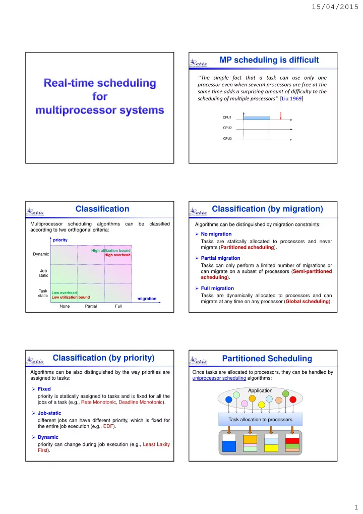
15/04/2015 MP scheduling is difficult “ The simple fact that a task can use only one processor even when several processors are free at the same time adds a surprising amount of difficulty to the scheduling of multiple processors ” [Liu 1969] CPU1 CPU2 CPU3 Classification Classification (by migration) Multiprocessor scheduling algorithms can be classified Algorithms can be distinguished by migration constraints: according to two orthogonal criteria:  No migration priority Tasks are statically allocated to processors and never migrate ( Partitioned scheduling ). High utilization bound Dynamic High overhead  Partial migration Tasks can only perform a limited number of migrations or Job can migrate on a subset of processors ( Semi-partitioned static scheduling ).  Full migration Task Low overhead Tasks are dynamically allocated to processors and can static Low utilization bound migration migrate at any time on any processor ( Global scheduling ). None Partial Full Classification (by priority) Partitioned Scheduling Algorithms can be also distinguished by the way priorities are Once tasks are allocated to processors, they can be handled by assigned to tasks: uniprocessor scheduling algorithms:  Fixed Application priority is statically assigned to tasks and is fixed for all the jobs of a task (e.g., Rate Monotonic, Deadline Monotonic).  Job-static Task allocation to processors different jobs can have different priority, which is fixed for the entire job execution (e.g., EDF).  Dynamic priority can change during job execution (e.g., Least Laxity First). 1

15/04/2015 Partitioned Scheduling Partitioned Scheduling Partitioned scheduling reduces to:  Each processor manages its own ready queue  The processor for each task is determined off-line Uniprocessor + Bin Packing  The processor cannot be changed at run time scheduling NP-hard in the Well known  4  1  1 strong sense P1 Task allocation Various heuristics used:  3  2  2 P2 FF, NF, BF, FFDU, BFDD, etc. Since migration is forbidden, processors may be underutilized.  5  5 P3 Global scheduling Global scheduling  The system manages a single queue of ready tasks Example (Global Rate Monotonic) C i T i  The processor is determined at run time  1  Consider the following task set: 3 6  During execution a task can migrate to another processor  2 7 10  3 8 12  The task set has to be scheduled on  4 6 15  1 P1 3 identical processors (m = 3)  5 3 18  Priority are assigned according to  5  4  3  2  1  2 P2 Rate Monotonic  3 P 1 > P 2 > P 3 > P 4 > P 5 P3 Global scheduling Global scheduling Work conserving scheduler Example (Global-RM)  The m highest priority tasks are always those executing. When a task finishes its execution (e.g.,  1 ), the next one in the queue (  4 ) is scheduled on the available CPU:  No processor is ever idle when a task is ready to execute.  1  4 P1 P1  5  4  3  2  1  2  5  4  3  2  2 P2 P2  3  3 P3 P3 2

15/04/2015 Global scheduling Global scheduling Example (Global-RM) Example (Global-RM) When a higher priority task arrives (e.g.,  1 ), it preempts When another task ends its execution (e.g.,  2 ), the the task with lowest priority among the executing ones (  4 ): preempted task (  4 ) can resume its execution. Note that  4 migrated  1  1 from P1 to P2 P1 P1  5  4  3  2  1  2  5  4  3  1  4 P2 P2  3  3 P3 P3 Global scheduling Global scheduling  1 (3, 6)  2 (7, 10)  3 (8, 12) Processor-level Task-level representation  4 (6, 15)  5 (3, 18) representation  1  1  4  1  2 (3,6) P1  2  2  4  1  4 (7,10) P2  3  3  5  3 (8,12) P3  1  1  2  4  5  4 all  3 (6,15) 0 2 4 6 8 10 12 14 16 18  5 (3,18) 0 2 4 6 8 10 12 14 16 18 Hybrid approaches Semi-partitioned scheduling Different restrictions can be imposed on task migration:  Tasks are statically allocated to processors, if possible.  Remaining tasks are split into chunks (subtasks), which  Job migration are allocated to different processors. Tasks are allowed to migrate, but only at jobs boundaries.  Semi-partitioned scheduling C i T i u i  51  1  5 Some tasks are statically allocated to processors, others 3 6 0.5  4  2  52 7 10 0.7 are split into chunks (subtasks) that are allocated to  3 9 15 0.6 different processors.  2  4  3 8 20 0.4  1  5  Clustered scheduling 15 30 0.5 A task can only migrate within a predefined subset of P1 P2 P3 U = 2.7 processors (cluster). 3

15/04/2015 Semi-partitioned scheduling Clustered scheduling  Note that subtasks are not independents,  A task can only migrate within a predefined subset of  51  52 but are subject to a precedence constraint: processors (cluster). This precedence must be managed! P1  3  2  1 Cluster 1 Task allocation  4  1  1 P1 P2  51  2  2 P2 P3  4  5 Cluster 2  52  3  3 P3 P4 Schedulability bound A negative result Given a set  of n periodic tasks with total utilization U to be The schedulability bound of global-EDF and global-RM is scheduled by an algorithms A on a set of m identical equal to 1, independently of the number m of available processors, find a bound U A (n,m) such that, processors. if U  U A (n,m), then  is schedulable by A. This means that given a platform of m identical A necessary condition processors, there exist applications with U > 1 that are A task set can be schedulable only if U  m. not schedulable by global-EDF and global-RM. In fact, it is clear that if U > m, the total demand in the To prove this result it suffices to identify an application  hyperperiod H will certainly exceed the total available time (that is UH > mH), hence some task will miss its deadline. with utilization U = 1+  (  is a constant arbitrarily small) that is not schedulable by global-EDF and global-RM. An algorithm A is optimal in the sense of schedulability iff U A (n,m) = m. Dhall's effect Partitioned C i T i U i C i T i U i  1  1 T  1  T  1  m processors m processors 1 EDF and RM produce 1 Note that a feasible  2  2 T  1  T  1  1 1 an unfeasible schedule partitioned schedule m+1 tasks . m+1 tasks . . . . with a total utilization . exists on just 2  m  m T  1 T  1 global schedule   1 1 arbitrarily close to 1 processors  m+1  m+1 T T 1 T T 1 P1 P1 T P2 P2 P3 Pm T 4

15/04/2015 Dhall's effect implications Global vs. partitioned On the other hand, there are task sets that are schedulable  Dhall's Effect shows the limitation of global EDF only with a global scheduler. and RM: both utilization bounds tend to 1, independently of the value of m. C i T i  1 Example: 1 2  Researchers lost interest in global scheduling for  2 2 3 ~25 years, since late 1990s.  3 2 3  Such a limitation is related to EDF and RM, not to  1  3  3  1  3 global scheduling in general. P1  2  1  2 P2 0 1 2 3 4 5 6 Global vs. partitioned Global vs. partitioned But there are also task sets that are schedulable only with a Example of unfeasible schedule with priorities: P 1 > P 2 > P 3 > P 4 partitioned scheduler. T i C i C i T i  1  1 4 6 Example: 4 6  2 7 12  2 7 12 P1  3  3 4 12 4 12 P2  4  4 misses 10 24  4 10 24 its deadline  1  3  1  3  1  3  1  3  1  3  1  1  3  1 P1 P1  2  4  2  4  2  3  4  2  3  4 P2 P2 0 2 4 6 8 10 12 14 16 18 20 22 24 0 2 4 6 8 10 12 14 16 18 20 22 24 All 4! = 24 global priority assignments lead to deadline miss. Global scheduling: pros & cons Evaluation metrics  Percentage of schedulable task sets Automatic load balance among processors – Over a randomly generated load Can better manage dynamic workloads – Depends on the task generation method Lower average response time (see queueing theory) More efficient reclaiming of unused processors  Processor speedup factor S More efficient overload management An algorithm A has a speedup factor S if any task set Lower number of preemptions feasible on a given platform can be scheduled by A on a platform in which all processors are S times faster. High migration cost: can be mitigated by proper HW (e.g.,  Run-time complexity MPCore’s Direct Data Intervention) Less schedulability results  Further research needed  Sustainability and predictability properties Schedulability is preserved for more relaxed constraints 5