Motivation Dramatic increase in digital data Privacy-Preserving - PowerPoint PPT Presentation

Motivation • Dramatic increase in digital data Privacy-Preserving Data Mining • World Wide Web • Growing Privacy Concerns Rakesh Agrawal Ramakrishnan Srikant A Surveys of web users IBM Almaden Research Center – 17% privacy fundamentalists, 56% pragmatic majority, 27% marginally concerned (Understanding net users' attitude about online privacy, April 99) Presented by Guiwen Hou – 82% said having privacy policy would matter (Freebies & Privacy: What net users think, July 99) 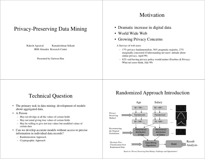Randomized Approach Introduction Technical Question Age Salary • The primary task in data mining: development of models 30 | 70K | ... 50 | 40K | ... ... about aggregated data. • A Person Privacy- Randomizer Randomizer Preserving – May not divulge at all the values of certain fields Method – May not mind giving true values of certain fields ... 65 | 20K | ... 25 | 60K | ... – May be willing to give not true values but modified values of certain data Reconstructing Reconstruct Reconstruct • Can we develop accurate models without access to precise the Original distribution distribution ... information in individual data records? Distribution of Age of Salary – Randomization Approach – Cryptographic Approach Result Decision-Tree Data Mining Model Analysis Classification Over Algorithms Randomized Data Based on “Privacy Preserving Data Mining: Challenges and Opportunities”

Talk Overview Privacy-Preserving Method • Value-Class Membership • Introduction Discretize continuous valued attributes. Values for an attribute are • Privacy-Preserving Method partitioned into a set of disjoint, mutually-exclusive classes. Instead of returning a true value, it returns the interval that the value lies. • Reconstructing the Original Distribution • Value Distortion • Decision-Tree Classification Over Add random component to data, return a value x i + r Instead of X i Randomized Data - Uniform - Gaussian • Experiment Result = • Conclusion and Future Work Based on R.Conway and D.Strip “select Partial Access to a Database”, In Proc, ACM Annual Conf. Quantifying Privacy Talk Overview Talk Overview • Measurement of how closely the original values of a modified attribute can be estimated. • Introduction • If it can be estimated with c% confidence that a value x lies in the interval [x1,x2], then the interval width (x2-x1) defines the amount of privacy at c% confidence • Privacy-Preserving Method level. • Reconstructing the Original Distribution • Discretization : Assumed that intervals are of equal width W - Problem • Uniform: random variable between [-a,a], The mean of the random variables is 0 - Reconstructing Procedure • Gaussian: The random variable has normal distribution, with mean u= 0 and stand deviation � - Reconstruction Algorithm - How does it work • Decision-Tree Classification Over Randomized Data • Experiment Result • Conclusion and Future Work

Reconstructing The Original Distribution (Procedure) Reconstructing The Original Distribution • Step1: Get single point density functions Problem: Use Bayes' rule for density functions • Original values x 1 , x 2 , ..., x n – from probability distribution X (unknown) • To hide these values, we use y 1 , y 2 , ..., y n – from probability distribution Y (known) • Given V 10 90 – x 1 +y 1 , x 2 +y 2 , ..., x n +y n (Perturbed Value) Age – the probability distribution of X+Y (known) Original distribution for Age Estimate the probability distribution of X. Probabilistic estimate of original value of V Based on “Privacy Preserving Data Mining: Challenges and Opportunities” Reconstructing The Original Distribution Reconstructing The Original Distribution (Bootstrapping) (Procedure) 0 := Uniform distribution + − • Step2 : Combine estimates of where point came j f X 1 n (( ) ) ( ) ∑ f x y a f a Y i i X ∞ from for all the points: j := 0 // Iteration number ∫ n + − j = (( ) ) ( ) f x y a f a i 1 Y i i X repeat − ∞ Compute new f X j+1 (a) based on f X j (a) (Bayes' rule) j := j+1 until (stopping criterion met) 10 90 Age Stopping Criterion: Difference between successive estimates becomes very small Based on “Privacy Preserving Data Mining: Challenges and Opportunities”

How well it works Talk Overview • Uniform random variable [-0.5, 0.5] • Introduction • Privacy-Preserving Method • Reconstructing the Original Distribution • Decision-Tree Classification Over Randomized Data - Decision Tree Algorithm - Demo a Decision Tree - Training using Randomized Data - Methods of building decision tree using Randomized Data • Experiment Result • Conclusion and Future Work Plateau Triangles Decision Tree Classification An Example of Decision Tree Classification: Given a set of classes, and a set of records in each class, develop a model that predicts the class of a new record . Partition(Data S) Begin if (most points in S are of the same class) then return; for each attribute A do evaluate splits on attribute A; Use best split to partition S into S1 and S2; Partition(S1); Partition(S2); End Initial call: Partition(TrainingData)

Selecting split point using “gini index” Selecting split point using “gini index”(cont.) We use the gini index to determine the goodness of a split. For a data set S containing ∑ j 2 examples from m classes, gini(S) = 1 - where p j is the relative frequency of P j SPLIT: Age <= 50 For S1: P(high) = 8/19 = 0.42 and P(low) = 11/19 = 0.58 class j in S. If a split divides S into two subsets S 1 and S 2 , the index of the divided data gini split (S) is given by gini split (S) = n1/n x gini(S 1 ) + n2/n x gini(S 2 ). | High | Low | Total For S2: P(high) = 11/21 = 0.52 and P(low) = 10/21 = 0.48 S1 (left) | 8 | 11 | 19 Gini(S1) = 1-[0.42x0.42 + 0.58x0.58] = 1-[0.18+0.34] = 1-0.52 = 0.48 Note that calculating this index requires only the distribution of the class values in S2 (right)| 11 | 10 | 21 Gini(S2) = 1-[0.52x0.52 + 0.48x0.48] = 1-[0.27+0.23] = 1-0.5 = 0.5 each of the partitions . Gini-Split(Age<=50) = 19/40 x 0.48 + 21/40 x 0.5 = 0.23 + 0.26 = 0.49 SPLIT: Salary <= 65K For S1: P(high) = 18/23 = 0.78 and P(low) = 5/23 = 0.22 | High | Low | Total For S2: P(high) = 1/17 = 0.06 and P(low) = 16/17 = 0.94 S1 (top) | 18 | 5 | 23 Gini(S1) = 1-[0.78x0.78 + 0.22x0.22] = 1-[0.61+0.05] = 1-0.66 = 0.34 S2 | 1 | 16 | 17 Gini(S2) = 1-[0.06x0.06 + 0.94x0.94] = 1-[0.004+0.884] = 1-0.89 = 0.11 (bottom) Gini-Split(Age<=50) = 23/40 x 0.34 + 17/40 x 0.11 = 0.20 + 0.05 = 0.25 Training using Randomized Data Training using Randomized Data (cont.) • Need to modify two key operations: • Determining split points: – Determining a split point. – Candidate splits are interval boundaries. – Partitioning the data. – Use statistics from the reconstructed distribution. • When and how do we reconstruct the original • Partitioning the data: distribution? – Reconstruction gives estimate of number of – Reconstruct using the whole data (globally) or points in each interval. – Reconstruct separately for each class? – Associate each data point with an interval by – Reconstruct once at the root node or reconstruct at sorting the values . every node?

Talk Overview Algorithms of Building Decision Tree • “Global” Algorithm • Introduction • Privacy-Preserving Method – Reconstruct for each attribute once at the beginning • Reconstructing the Original Distribution • “By Class” Algorithm • Experiment Result – For each attribute, first split by class, then reconstruct - Experimental Methodology separately for each class. - Synthetic Data Functions • “Local” Algorithm - Classification Accuracy – As in By Class, split by class and reconstruct - Accuracy vs. Randomization Level separately for each class. • Conclusion and Future Work – However, reconstruct at each node (not just once). Synthetic Data Functions Experimental Methodology Class A if function is true, Class B otherwise • F1 • Compare accuracy against (age < 40) or ((60 <= age) – Original: unperturbed data without randomization. • F2 ((age < 40) and (50K <= salary <= 100K)) or – Randomized: perturbed data but without making any ((40 <= age < 60) and (75K <= salary <= 125K)) or corrections for randomization. ((age >= 60) and (25K <= salary <= 75K)) • F3 • Test data not randomized. ((age < 40) and (((elevel in [0..1]) and (25K <= salary <= 75K)) or • Synthetic data generator from [AGI+92]. ((elevel in [2..3]) and (50K <= salary <= 100K))) or ((40 <= age < 60) and ... • Training set of 100,000 records, a test set of 5,000 records. • F4 split equally between the two classes. (0.67 x (salary+commission) - 0.2 x loan - 10K) > 0 • F5 (0.67 x (salary+commission) - 0.2 x loan +0.2 x equity - 10K) > 0 Where equity = 0.1 x hvalue x max(hyears – 20.0 )

Classification accuracy Privacy Level Uniform Example: Privacy Level for Age[10,90] Given a perturbed value 40 95% confidence that true value lies in [30,50] (Interval Width : 20) /(Range : 80) = 25% privacy level Privacy Level: 25% of Attribute Range Privacy Level: 100% of Attribute Range 25% privacy level @ 95% confidence Accuracy vs. Privacy Level Acceptable loss in accuracy Acceptable loss in accuracy 100% Privacy Level 100 90 Original 80 Accuracy Randomized 70 ByClass 60 Global 50 Fn 1 Fn 3 40 Fn 1 Fn 2 Fn 3 Fn 4 Fn 5