Motivation Scanners to obtain virtual 3D shapes Surface - - PDF document

1

CS101b - Meshing

1

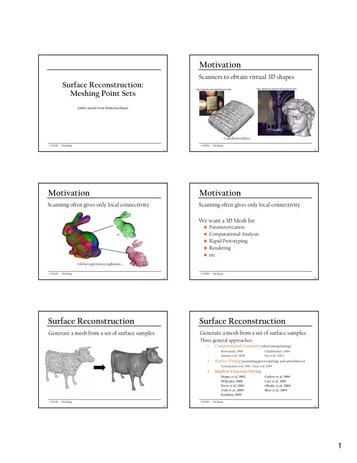
Surface Reconstruction: Meshing Point Sets

(slides mostly from Misha Kazhdan)

CS101b - Meshing

2

Motivation

Scanners to obtain virtual 3D shapes

http://www.jhu.edu/digitalhammurabi/ http://graphics.stanford.edu/projects/mich/

Cuneiform tablets

CS101b - Meshing

3

Motivation

Scanning often gives only local connectivity

Global registration nightmare….

CS101b - Meshing

4

Motivation

Scanning often gives only local connectivity We want a 3D Mesh for:

Parameterization Computational Analysis Rapid Prototyping Rendering etc

CS101b - Meshing

5

Surface Reconstruction

Generate a mesh from a set of surface samples

CS101b - Meshing

6

Surface Reconstruction

Generate a mesh from a set of surface samples

Three general approaches:

1.

Computational Geometry (often interpolating)

Boissonnat, 1984 Edelsbrunner, 1984 Amenta et al., 1998 Dey et al., 2003 2.

Surface Fitting (assuming given topology and smoothness)

Terzopoulos et al., 1991 Chen et al., 1995 3.

Implicit Function Fitting

Hoppe et al., 1992 Curless et al., 1996 Whitaker, 1998 Carr et al., 2001 Davis et al., 2002 Ohtake et al., 2004 Turk et al., 2004 Shen et al., 2004 Kazhdan, 2005

2

CS101b - Meshing

7

Implicit Function Approach

Define a function with value less than zero

• utside the model and

greater than zero inside

< 0

> 0

CS101b - Meshing

8

Implicit Function Approach

Define a function with value less than zero

• utside the model and

greater than zero inside Extract the zero-set

< 0

> 0

CS101b - Meshing

9

Accurate Reconstructions

To extract fine surface detail, represent the implicit function at a high resolution. Limitation of convolution: Regular voxel grids have complexity proportional to the volume not the surface.

Kazhdan 2005, FFT Reconstruction

CS101b - Meshing

10

Accurate Reconstructions

An accurate representation is (often) only required near the surface. Limitations of RBF:

Solve large, dense linear systems Hard to control away from samples

Carr et al. 2001, FastRBF

CS101b - Meshing

11

Accurate Reconstructions

An accurate representation is (often) only required near the surface. Limitations of MPU:

Solve large, quite-dense linear systems Hard to control away from samples Local solutions are more susceptible to noise

Ohtake et al. 2004, MPU

CS101b - Meshing

12

Outline

Introduction Approach

Key Ideas of Poisson Reconstruction Implementation

Results Conclusion

Kazhdan, Bolitho, and Hoppe ‘06

3

CS101b - Meshing

13

Indicator Function

We reconstruct the surface of the model by solving for the “indicator” function of the shape. ( )

⎩ ⎨ ⎧ ∉ ∈ = M p M p p

M

if if 1 χ χM

Indicator function

1 1 1

CS101b - Meshing

14

Challenge

How to construct the indicator function?

χM

Indicator function Oriented points (points+normals)

CS101b - Meshing

15

Gradient vs Normal

There is a relationship between the normal field and the gradient of indicator fct

smoothed indicator function

∇χM

Indicator gradient

Oriented points (points+normals)

CS101b - Meshing

16

Integration as a Poisson Problem

Represent input data by a vector field Find the function whose gradient best approximates : Applying the divergence operator: Poisson problem!

χ

V r

2

) ( min V r − ∇χ

χ

( )

V V r r ⋅ ∇ = Δ ⇔ ⋅ ∇ = ∇ ⋅ ∇ χ χ

V r

CS101b - Meshing

17

Note

Simple L2 projection (see, e.g., Tong et al) :

Now use integration by part and you get Poisson!

CS101b - Meshing

18

Simple Implementation

Given the Points:

Set octree Compute vector field Compute indicator function Extract isosurface

4

CS101b - Meshing

19

Implementation: Adapted Octree

Given the Points:

Set octree Compute vector field Compute indicator function Extract iso-surface

CS101b - Meshing

20

Implementation: Vector Field

Given the Points:

Set octree Compute vector field

Define a function space Splat the samples

Compute indicator function Extract iso-surface

CS101b - Meshing

21

Implementation: Vector Field

Given the Points:

Set octree Compute vector field

Define a function space Splat the samples

Compute indicator function Extract iso-surface

CS101b - Meshing

22

Implementation: Vector Field

Given the Points:

Set octree Compute vector field

Define a function space Splat the samples

Compute indicator function Extract iso-surface

CS101b - Meshing

23

Implementation: Vector Field

Given the Points:

Set octree Compute vector field

Define a function space Splat the samples

Compute indicator function Extract iso-surface

CS101b - Meshing

24

Implementation: Vector Field

Given the Points:

Set octree Compute vector field

Define a function basis Splat the samples

Compute indicator function Extract iso-surface

5

CS101b - Meshing

25

Implementation: Vector Field

Given the Points:

Set octree Compute vector field

Define a function basis Splat the samples

Compute indicator function Extract iso-surface

CS101b - Meshing

26

Implementation: Vector Field

Given the Points:

Set octree Compute vector field

Define a function basis Splat the samples

Compute indicator function Extract iso-surface

CS101b - Meshing

27

Implementation: Vector Field

Given the Points:

Set octree Compute vector field

Define a function space Splat the samples

Compute indicator function Extract iso-surface

CS101b - Meshing

28

Implementation: Indicator Fct

Given the Points:

Set octree Compute vector field Compute indicator function

Compute divergence Solve Poisson equation

Extract iso-surface

CS101b - Meshing

29

Implementation: Indicator Fct

Given the Points:

Set octree Compute vector field Compute indicator function

Compute divergence Solve Poisson equation

Extract iso-surface

CS101b - Meshing

30

Implementation: Indicator Fct

Given the Points:

Set octree Compute vector field Compute indicator function

Compute divergence Solve Poisson equation

Extract iso-surface

6

CS101b - Meshing

31

Implementation: Extraction

Given the Points:

Set octree Compute vector field Compute indicator function Extract iso-surface

CS101b - Meshing

32

Outline

Introduction Approach Results

Evaluation of Poisson approach Comparison to related work

Conclusion

CS101b - Meshing

33

Michelangelo’s David

215 million data points

• from 1000 scans

22 million triangle reconstruction Compute Time: 2.1 hours Peak Memory: 6600MB

CS101b - Meshing

34

David – Chisel marks

CS101b - Meshing

35

David – Drill Marks

CS101b - Meshing

36

David – Eye

7

CS101b - Meshing

37

Scalability – Buddha Model

1 00 200 300 400 500 600 700 800 900 1 00,000 200,000 300,000 400,000 500,000 600,000 700,000 800,000 Triangles Time (s) / Peak Memory (MB ) Time Taken Peak Memory Usage

CS101b - Meshing

38

Stanford Bunny

Power Crust FastRBF MPU VRIP FFT Reconstruction Poisson

CS101b - Meshing

39

Medical Data

Arbitrary topology

CS101b - Meshing

40

VRIP Comparison

VRIP Poisson

CS101b - Meshing

41

FFT Reconstruction Comparison

FFT: Fixed resolution

Low Resolution High Resolution

CS101b - Meshing

42

FFT Reconstruction Comparison

Low Resolution High Resolution

FFT: Fixed resolution

8

CS101b - Meshing

43 Low Resolution High Resolution

FFT Reconstruction Comparison

FFT: Fixed resolution

CS101b - Meshing

44

FFT Reconstruction Comparison

Poisson: Adaptive resolution

CS101b - Meshing

45

FFT Reconstruction Comparison

Poisson: Adaptive resolution

CS101b - Meshing

46

Comparison

310 263 911,390 Poisson Reconst. 1684 125 910,320 Kazhdan 2005 186 86 1,038,055 VRIP 330 70 950,562 Hoppe et al 1992 260 28 925,240 MPU 796 4919 1,798,154 FastRBF 544 892 272,662 Robust Cocone 2653 380 554,332 Power Crust

Mem (MB) Time (s) Triangles Method

=

CS101b - Meshing

47

Conclusion

Theoretical Contributions:

Relate oriented samples to indicator gradient Express reconstruction as a Poisson problem easily solved via CG

Empirical Advantages:

Is robust to noise (because mostly global) Adapts to the sampling density Can handle large models

Empirical Flaws:

noise creates spurious connected components