Motivation Many applications of databases manipulate geographical - - PDF document

SLIDE 1

Multidimensional (Spatial) Indexing

CS5208 – Spatial Indexing 1

Motivation

• Many applications of databases manipulate geographical (2-d)
• data. Others involve large number of dimensions
• Examples:

– location of restaurants in a city. – Map data: zones, county lines, rivers, lakes, etc. (Data has spatial extent) – Sales information described by store, day, item, color, size,

• etc. Sale = point in multidimensional space.

– Student described by age, zipcode, marital status.

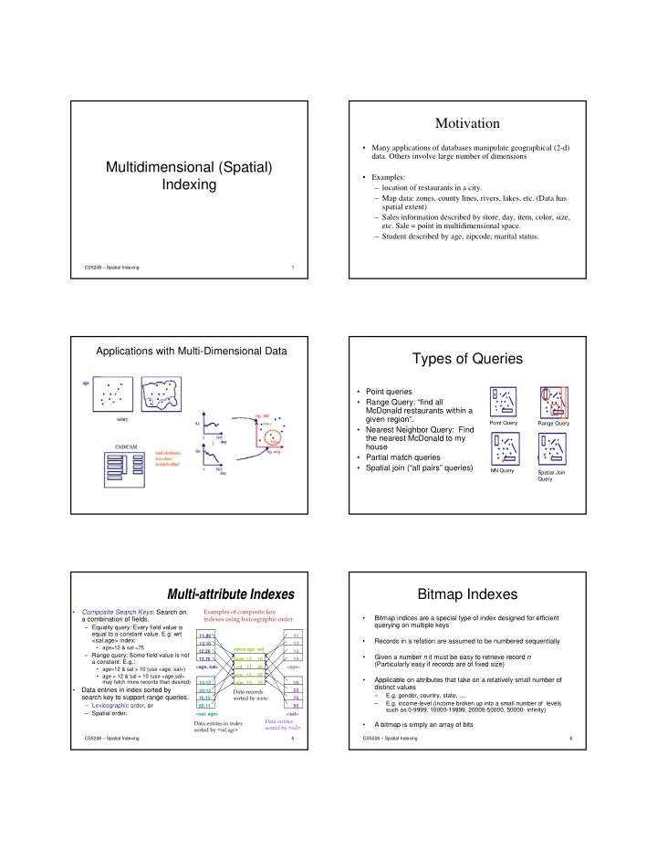
Applications with Multi-Dimensional Data

Types of Queries

Point Query Range Query NN Query Spatial Join Query

• Point queries
• Range Query: “find all

McDonald restaurants within a given region”.

• Nearest Neighbor Query: Find

the nearest McDonald to my house

• Partial match queries
• Spatial join (“all pairs” queries)

CS5208 – Spatial Indexing 5

Multi-attribute Indexes

• Composite Search Keys: Search on

a combination of fields.

– Equality query: Every field value is equal to a constant value. E.g. wrt <sal,age> index:

• age=12 & sal =75

– Range query: Some field value is not a constant. E.g.:

• age=12 & sal > 10 (use <age, sal>)
• age < 12 & sal = 10 (use <age,sal>

may fetch more records than desired)

• Data entries in index sorted by

search key to support range queries.

– Lexicographic order, or – Spatial order.

sue 13 75 bob cal joe 12 10 20 80 11 12 name age sal <sal, age> <age, sal> <age> <sal> 12,20 12,10 11,80 13,75 20,12 10,12 75,13 80,11 11 12 12 13 10 20 75 80

Data records sorted by name Data entries in index sorted by <sal,age> Data entries sorted by <sal>

Examples of composite key indexes using lexicographic order.

CS5208 – Spatial Indexing 6

Bitmap Indexes

• Bitmap indices are a special type of index designed for efficient

querying on multiple keys

• Records in a relation are assumed to be numbered sequentially
• Given a number n it must be easy to retrieve record n

(Particularly easy if records are of fixed size)

• Applicable on attributes that take on a relatively small number of

distinct values

– E.g. gender, country, state, … – E.g. income-level (income broken up into a small number of levels such as 0-9999, 10000-19999, 20000-50000, 50000- infinity)

• A bitmap is simply an array of bits

SLIDE 2

CS5208 – Spatial Indexing 7

Use of Bitmap Indexes: Example

• In its simplest form, a bitmap index on an attribute has a bitmap for

each value of the attribute

– Bitmap has as many bits as records – In a bitmap for value v, the bit for a record is 1 if the record has the value v for the attribute, and is 0 otherwise – Size = nm bits where n is the #records, m is the #distinct values

CS5208 – Spatial Indexing 8

Bitmap Indexes (Cont.)

• Queries are answered using logical (bitwise) operations

– Intersection (and) – Union (or) – Complementation (not)

• Each operation takes two bitmaps of the same size and applies the
• peration on corresponding bits to get the result bitmap

– Males with income level L1

• 10010 AND 10100 = 10000
• Can then retrieve required tuples
• Counting number of matching tuples is even faster
• Range queries?

– Age IN [30,40] AND Salary IN [10k,20k]

CS5208 – Spatial Indexing 9

Compressed Bitmaps

• If n and m are large, then nm bits may incur high

I/O

• Compress the bitmap – run-length encoding

– A sequence of i 0’s followed by a 1 (run) is represented by some binary encoding of the integer i – A number i is represented by (log2i-1) 1-bit (indicates the number of bits required to represent i) and a single 0, followed by its binary value

• E.g., 13 = 1101 (binary) is represented as

111 0 1101

• Exceptions: i = 0 is 00; i = 1 is 01

– Every run incurs 2 log2i bits

log13-1 13

CS5208 – Spatial Indexing 10

Compressed Bitmap (Cont.)

• Consider 0000000000000110001

– The encoded sequence is …

• Now consider 000000010000 (i.e., n = 12)
• What is the compressed bitmap?
• Decode 110111

– What about the (missing) 0’s?

CS5208 – Spatial Indexing 11

Operating on Compressed Bitmap

• Need to decode first, then perform the

bitwise operations

• But can be done incrementally
• Suppose we ORed encodings:

0 0 1 1 0 1 1 1 1 1 0 1 1 1

7 00000001 OUTPUT:

CS5208 – Spatial Indexing 12

Operating on Compressed Bitmap

• Need to decode first, then perform the

bitwise operations

• But can be done incrementally
• Suppose we ORed encodings:

0 0 1 1 0 1 1 1 1 1 0 1 1 1

7 7 00000001 00000001

0 0 0 0 0 0 0 1

OUTPUT:

SLIDE 3

CS5208 – Spatial Indexing 13

Operating on Compressed Bitmap

• Need to decode first, then perform the

bitwise operations

• But can be done incrementally
• Suppose we ORed encodings:

0 0 1 1 0 1 1 1 1 1 0 1 1 1

7 7 00000001 00000001

0 0 0 0 0 0 0 1 1

OUTPUT:

Why spatial index methods (SAMs)?

• B-tree & hash tables

– Guarantee the number of I/O operations is respectively logarithmic and constant with respect to the collection’s size – Index a collection on a key – Rely on a total order on the key domain, the order

• f natural numbers, or the lexicographic order on

strings

• There is no such total order for

multidimensional objects and geometric

• bjects with spatial extent
• SAMs were designed to try as much as

possible to preserve spatial object proximity

CS5208 – Spatial Indexing 14

Multidimensional Indexing Structures

• Space-Based structures:

– Partition the embedding Space into rectangular cells – Independent from the distribution of the objects – Objects are mapped to the cells based on some geometric criterion – Eg: Grid file, Buddy-tree, KDB-tree

• Data-Based structures:

– Organize by partitioning the set of objects based on spatial proximity such that each group can fit into a page – Adapt to the objects’ distribution – Eg. R-tree, R* tree, R+ tree

• Mapping

– Transform the data into lower dimensional space – E.g., space filling curve

CS5208 – Spatial Indexing 15

Grid File: A Space-based Approach

• Start with one bucket

for the whole space.

• Select dividers along

each dimension. Partition space into cells

• Dividers cut all the

way

CS5208 – Spatial Indexing 16

Grid File

• Each cell corresponds

to 1 disk page.

• Many cells can point

to the same page.

• Cell directory

potentially exponential in the number of dimensions

CS5208 – Spatial Indexing 17

Grid File Implementation

• Dynamic structure using a grid directory

– Grid array: a 2 dimensional array with pointers to buckets (this array can be large, disk resident) G(0,…, nx-1, 0, …, ny-1) – Linear scales: Two 1 dimensional arrays that used to access the grid array (main memory) X(0, …, nx-1), Y(0, …, ny-1)

CS5208 – Spatial Indexing 18

SLIDE 4

Example

Linear scale X Linear scale Y Grid Directory Buckets/Disk Blocks

CS5208 – Spatial Indexing 19

Grid File Search

• Exact Match Search: at most 2 I/Os assuming linear scales fit in

memory.

– First use linear scales to determine the index into the cell directory – access the cell directory to retrieve the bucket address (may cause 1 I/O if cell directory does not fit in memory) – access the appropriate bucket (1 I/O)

• Range Queries:

– use linear scales to determine the index into the cell directory. – Access the cell directory to retrieve the bucket addresses of buckets to visit. – Access the buckets.

• Nearest Neighbor Queries:

– Search the bucket corresponding to the cell in which the query point P belongs – If we find at least one point, we have a candidate Q for the NN – However, it is possible that there are points in adjacent buckets that are closer to P than Q is; in this case, we need to search these buckets.

CS5208 – Spatial Indexing 20

Grid File Insertions

• Determine the bucket into which insertion must occur.
• If space in bucket, insert.
• Else, split bucket (alternatively: use overflow buckets?)

– how to choose a good dimension to split? – ans: create convex regions for buckets.

• If bucket split causes a cell directory to split do so and

adjust linear scales.

– When does the cell directory not split?

• insertion of these new entries potentially requires a

complete reorganization of the cell directory--- expensive!!!

CS5208 – Spatial Indexing 21

Grid File Deletions

• Deletions may decrease the space utilization.

Merge buckets

• We need to decide which cells to merge and

a merging threshold

• Buddy system and neighbor system

– A bucket can merge with only one buddy in each dimension – Merge adjacent regions if the result is a rectangle

CS5208 – Spatial Indexing 22 CS5208 – Spatial Indexing 23

R-Trees: A Data-based Approach

• R-trees
• N-dimensional extension of B+-trees
• Height-balanced, all leaf nodes appear at the same level, each

node has between t and M entries

• useful for indexing sets of points, rectangles and other

polygons.

• Basic idea: generalize the notion of a one-dimensional

interval associated with each B+ -tree node to an N-dimensional interval, that is, an N-dimensional rectangle.

• Will consider only the two-dimensional case (N = 2)
• generalization for N > 2 is straightforward

CS5208 – Spatial Indexing 24

Note that we only need two points to describe an MBR, we typically use lower left, and upper right.

MBR = {(L.x,L.y)(U.x,U.y)}

Bounding Rectangle

• Suppose we have a cluster of points in 2-D space...

– We can build a “box” around points. The smallest box (which is axis parallel) that contains all the points is called a Minimum Bounding Rectangle (MBR)

• also known as minimum bounding box

SLIDE 5

CS5208 – Spatial Indexing 25

R-Tree: Clustering by Proximity

2 4 6 8 10 2 4 6 8 10 x axis y axis b c a

E

3

a b c d e E1 E2 E3 E4 E5 Root E1 E2 E3 E4 f g h E5

d e f g h i j k l m

l m E7 i j k E6 E6 E7

Minimum Bounding Rectangle (MBR)

CS5208 – Spatial Indexing 26

R-Tree

2 4 6 8 10 2 4 6 8 10 x axis y axis b c a

E

3 d e f g h i j k l m

E

4

E

5

E

6

E

7

a b c d e E1 E2 E3 E4 E5 Root E1 E2 E3 E4 f g h E5 l m E7 i j k E6 E6 E7

27

R-Tree

2 4 6 8 10 2 4 6 8 10 x axis y axis b c a

E

1 d e f g h i j k l m

E

2

a b c d e E1 E2 E3 E4 E5 Root E1 E2 E3 E4 f g h E5 l m E7 i j k E6 E6 E7

28

R-Tree

2 4 6 8 10 2 4 6 8 10 x axis y axis b c a

E

1 d e f g h i j k l m

E

2

a b c d e E1 E2 E3 E4 E5 Root E1 E2 E3 E4 f g h E5 l m E7 i j k E6 E6 E7

CS5208 – Spatial Indexing 29

R Trees (Cont.)

A rectangular bounding box (a.k.a. MBR) is

associated with each tree node.

Bounding box of a leaf node is a minimum sized

rectangle that contains all the points associated with the leaf node.

The bounding box associated with a non-leaf

node contains the bounding box associated with all its children.

Bounding box of a node serves as its key in its

parent node (if any)

Bounding boxes of children of a node are allowed

to overlap

CS5208 – Spatial Indexing

R-Tree structure

• leaf entry = <object>

– An object may have extent.

• index entry = <MBR, ptr to child node>

– MBR of all objects in the subtree.

• Observation: if range query, Q, does not intersect

an MBR, no object in the sub-tree is inside Q.

Q MBR

30

SLIDE 6

CS5208 – Spatial Indexing

Range query

Start at root.

• 1. If current node is non-leaf, for each

entry <E, ptr>, if box E overlaps Q, search subtree identified by ptr.

• 2. If current node is leaf, for every object in

the leaf page, report if contained in Q.

Can be very inefficient in worst case since multiple paths may need to be searched but works acceptably in practice.

31

Range Query: Given a query box Q, find all points enclosed by Q

32

Range Query

2 4 6 8 10 2 4 6 8 10 x axis y axis b c a

E

1 d e f g h i j k l m

E

2

a b c d e E1 E2 E3 E4 E5 Root E1 E2 E3 E4 f g h E5 l m E7 i j k E6 E6 E7

33

Range Query

2 4 6 8 10 2 4 6 8 10 x axis y axis b c a

E

1 d e f g h i j k l m

E

2

a b c d e E1 E2 E3 E4 E5 Root E1 E2 E3 E4 f g h E5 l m E7 i j k E6 E6 E7

CS5208 – Spatial Indexing

Insert object o

• Start at root and go down to “best-fit” leaf L.

– Go to child whose box needs least enlargement to cover o; resolve ties by going to smallest area child.

• If best-fit leaf L has space, insert entry, adjust

bounding boxes starting from the leaf upwards

• Otherwise, split L into L1 and L2.

– Adjust entry for L in its parent so that the box now covers (only) L1. – Add an entry (in the parent node of L) for L2. (This could cause the parent node to recursively split.)

34 35

E.g. 1: no split, no enlargement

2 4 6 8 10 2 4 6 8 10 x axis y axis b c a

E

1 d e f g h i j k l m

E

2

a b c d e E1 E2 E3 E4 E5 Root E1 E2 E3 E4 f g h E5 l m E7 i j k E6 E6 E7

insert o

• 36

E.g. 2: no split, but enlargement

2 4 6 8 10 2 4 6 8 10 x axis y axis b c a

E

1 d e f g h i j k l m

E

2

a b c d e E1 E2 E3 E4 E5 Root E1 E2 E3 E4 f g h E5 l m E7 i j k E6 E6 E7

insert o

SLIDE 7

37

E.g. 2: no split, but enlargement

2 4 6 8 10 2 4 6 8 10 x axis y axis b c a

E

1 d e f g h i j k l m

E’

2

a b c d e E1 E’ 2 E3 E4 E5 Root E1 E’ 2 E3 E4 f g h E5 l m E7 i j k E6 E6 E’ 7

insert o

• CS5208 – Spatial Indexing

Insert object o

• Start at root and go down to “best-fit” leaf L.

– Go to child whose box needs least enlargement to cover o; resolve ties by going to smallest area child.

• If best-fit leaf L has space, insert entry, adjust

bounding boxes starting from the leaf upwards

• Otherwise, split L into L1 and L2.

– Adjust entry for L in its parent so that the box now covers (only) L1. – Add an entry (in the parent node of L) for L2. (This could cause the parent node to recursively split.)

38 39

E.g. 3: split

2 4 6 8 10 2 4 6 8 10 x axis y axis b c a

E

1 d e f g h i j k l m

E

2

a b c d e E1 E2 E3 E4 E5 Root E1 E2 E3 E4 f g h E5 l m E7 i j k E6 E6 E7

insert o

• 40

E.g. 3: split

2 4 6 8 10 2 4 6 8 10 x axis y axis b c a

E

1 d e f g h i j k l m

E

2

a b c d e E1 E2 E3 E4 E5 Root E1 E2 E3 E4 f g h E5 l m E7 i

• j

E6 E6 E7 k

• E’

6

CS5208 – Spatial Indexing

Splitting a Node During Insertion

• The entries in node L plus the newly inserted

entry must be distributed between L1 and L2.

• Goal is to reduce likelihood of both L1 and L2

being searched on subsequent queries.

• Idea: Redistribute so as to minimize area of L1

plus area of L2.

Exhaustive algorithm is too slow; quadratic and linear heuristics are described in the paper.

41 CS5208 – Spatial Indexing 42

Quadratic Split

• Quadratic split divides the entries in a node into two new nodes

as follows

• 1. Find pair of entries with “maximum separation”
• that is, the pair such that the bounding box of the two

would have the maximum wasted space (area of bounding box – sum of areas of two entries)

• 2. Place these entries in two new nodes
• 3. Repeatedly find an entry and assign it to one of the nodes
• Calculate d1 = the area increase required in the MBR of one node to

include the entry. Calculate d2 analogously for the other node

• Choose the entry with the maximum difference between d1 and d2
• Add It to the node whose MBR will have to be enlarged least to

accommodate It. Resolve ties by adding the entry to the node with the smallest area, then to the one with the fewer entries, then to either

• 4. Stop when half the entries have been added to one node
• Then assign remaining entries to the other node

SLIDE 8

Node Splitting R Node Splitting R-

• trees

trees

CS5208 – Spatial Indexing 43

Node Splitting R Node Splitting R-

• trees

trees

CS5208 – Spatial Indexing 44 CS5208 – Spatial Indexing 45

Deleting in R-Trees

• Deletion of an entry in an R-tree done

much like a B+-tree deletion.

– In case of underfull node, borrow entries from a sibling if possible, else merging sibling nodes – Alternative approach removes all entries from the underfull node, deletes the node, then reinserts all entries

NN search: Best-First Algorithm

• Global order

– Use only MINDIST – Maintain distance to all entries in a common Priority Queue – Repeat

• Inspect the next MBR in the list
• Add the children to the list and reorder

– Until all remaining MBRs can be pruned

CS5208 – Spatial Indexing 46

MINDIST

• MINDIST(P, R) is the minimum distance between a point

P and a rectangle R

• If the point is inside R, then MINDIST=0
• If P is outside of R, MINDIST is the distance of P to the

closest point of R (one point of the perimeter)

ri = li if pi < li = ui if pi > ui = pi otherwise p p p R l u

MINDIST = 0

∑

=

− =

d i i i

r p R P MINDIST

1 2

) ( ) , (

l=(l1, l2, …, ld) u=(u1, u2, …, ud)

) , ( ) , ( ,

• P

R P MINDIST R

• ≤

∈ ∀

CS5208 – Spatial Indexing 47

Nearest Neighbor Search (NN) with R-Trees

E

2 4 6 8 10 2 4 6 8 10 x axis y axis b

E

f query point

• mitted

1

E

2 e d c a h g

E

3

E

5

E

6

E

4

E7

8 search region contents

E

9 i E 1 1 E 2 2

Visit Root

E 13 7

follow E

1 E 2 2 E 5 4 E 5 5 E 8 3 E 9 6 E 8 3

Action Heap follow E

2 E 2 8 E 5 4 E 5 5 E 8 3 E 9 6

follow E

8

Report h and terminate

E 17 9 E 13 7 E 5 4 E 5 5 E 8 3 E 9 6 E 17 9

Result {empty} {empty} {empty} {(h,

2 )}

a 5 b 13 c 18 d 13 e 13 f 10 h 2 g 13 E1 1 E2 2 E3 8 E4 5 E5 5 E6 9 E7 13 E8 2 Root E9 17 i 10 E1 E2 E 4 E5 E8

i 10 E 5 4 E 5 5 E 8 3 E 9 6 E 13 7 g 13

CS5208 – Spatial Indexing 48

SLIDE 9

The NN Search Algorithm

Initialize PQ (priority queue) InesrtQueue(PQ, Root) While not IsEmpty(PQ)

R= Dequeue(PQ) If R is an object

Report R and exit (done!)

If R is a leaf page node

For each O in R, compute the Actual-Dists, InsertQueue(PQ, O)

If R is an index node

For each MBR C, compute MINDIST, insert into PQ

CS5208 – Spatial Indexing 49

K-NN search

• Keep the sorted buffer of at most k current nearest

neighbors

• Pruning is done using the k-th distance

CS5208 – Spatial Indexing 50

Space Filling Curves: Mapping Based Methods

• Assumption: att. values can be

represented with some fixed # of bits

• Space domain on each dimension: 2k

values

• Linearize the domain
• Each point can be represented by a single

dimensional value

CS5208 – Spatial Indexing 51

Z-ordering

00 01 10 11 00 01 10 11

CS5208 – Spatial Indexing 52

Z-ordering

• The z-value is obtained by interleaving the bits

CS5208 – Spatial Indexing 53

Z-ordering

• z-values can be indexed using B+-trees

– All commercial systems support B+-tree (no coding/debugging, concurrency and recovery support, etc)

CS5208 – Spatial Indexing 54

SLIDE 10

• Point queries: e.g., find city at (0,3)
• Find z-value; search B-tree

Z-ordering

CS5208 – Spatial Indexing 55

• Range queries?
• Compute ranges of z-values; use B-tree

Z-ordering

CS5208 – Spatial Indexing 56

Z-ordering

• Range queries?
• Compute ranges of z-values; use B-tree
• To reduce # of qualifying of ranges: Augment the query
• What’s the overhead?

CS5208 – Spatial Indexing 57

• Range queries - how to break a query into ranges?
• Recursively, quadtree-style; decompose only

non-full quadrants

Z-ordering

CS5208 – Spatial Indexing 58

• k-nn queries, e.g., 1-nn:
• Traverse B-tree; find nn wrt z-values and …

Z-ordering

ask a range query.

CS5208 – Spatial Indexing 59

Summary

• Many applications operate on multi-

dimensional data

• Advanced techniques are required
• Paradigm

– Space-partitioning – Data-partitioning – Mapping

CS5208 – Spatial Indexing 60