Mortality shifts and mortality compression in Norway 1900-2100: - PDF document

Work in progress. Do not cite or quote. Mortality shifts and mortality compression in Norway 1900-2100: empirical and predicted period and cohort life tables Nico Keilman, University of Oslo Dinh Quang Pham, Statistics Norway Astri Syse, Statistics Norway We explore mortality shifts and the compression of mortality in Norwegian men and women born in the period 1900-1990. We compare those patterns with shifts and compression based on period life tables. The data for the period 1900-2015 are empirically observed. For the years 2016-2100 the information comes from Stat istics Norway’s mortality projections. We analyse the mean age at death (life expectancy), as well as the median and modal ages at death. All three characterize shifts in mortality. 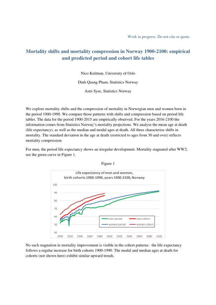The standard deviation in the age at death (restricted to ages from 30 and over) reflects mortality compression. For men, the period life expectancy shows an irregular development. Mortality stagnated after WW2; see the green curve in Figure 1. Figure 1 Life expectancy of men and women, birth cohorts 1900-1990, years 1900-2100, Norway 100 90 80 70 60 men period men cohort 50 women period women cohort 40 1900 1920 1940 1960 1980 2000 2020 2040 2060 2080 2100 No such stagnation in mortality improvement is visible in the cohort patterns: the life expectancy follows a regular increase for birth cohorts 1900-1990. The modal and median ages at death for cohorts (not shown here) exhibit similar upward trends.

Period data for the standard deviation (Figure 2) suggest a decompression of mortality in men after WW2. Cohort data in Figure 2 show very little change for cohorts 1900-1915, but a clear compression is visible for later cohorts. Figure 2 Standard deviation in age at death, men and women, birth cohorts 1900-1990, years 1900-2100, Norway 20 18 16 14 12 10 8 6 4 men period men cohort 2 women period women cohort 0 1900 1920 1940 1960 1980 2000 2020 2040 2060 2080 2100 NB. Standard deviation restricted to ages 30 and over. For women the cohort patterns in Figures 1 and 2 are very regular, signalling a continuous compression of mortality around an ever-increasing mean age at death. We have developed expressions that link cohort mortality to period mortality. With these, we can answer questions about mortality shifts and mortality compression such as - why does cohort life expectancy increase faster than period life expectancy? - why do cohort standard deviations fall steeper than period standard deviations? We build on earlier work by others, such as Canudas-Romo, V., Schoen, R. (2005) Age-specific contributions to changes in the period and the cohort life expectancy. Demographic Research 13(3): 63-82. Ediev, D. (2013) Mortality compression in period life tables hides decompression in birth cohorts in low-mortality countries. Genus 69(2):53-84. Wilmoth, J. (2005) On the relationship between period and cohort mortality. Demographic Research 13(3): 231-280. Goldstein, J., Wachter, K. (2006) Relationships between period and cohort life expectancy: Gaps and lags. Population Studies 60(3): 257-269. Missov, T.I., Lennart, A. (2011) Linking period and cohort life-expectancy linear increases in Gompertz proportional hazards models. Demographic Research 24(19): 455-468.

Our contribution is that we present a simple unified framework for analytical expressions for mortality shifts and mortality compression in period and cohort life tables. We focus on the age at death distribution (AADD) in a life table. This corresponds with the d x -column in the life table, provided that that the radix l 0 equals 1. Notation: V k [ t ] is the non-centered moment of order k of the period AADD  V 1 [ t ] is the period life expectancy in year t . W k [ t ] is the non-centered moment of order k of the cohort AADD  W 1 [ t ] is the cohort life expectancy for the cohort born in year t . The general expression is with A k and B k constants to be estimated from data, given k . The upper index ( i ) denotes derivation with respect to time. Note that we obtain Ryder’s translation formulae when A k = 0 and B k = 1. Findings for life expectancies (assuming linear cohort life expectancy). Finding 1 Period life expectancy in year t in which cohort born year g reaches its own life expectancy is Cohort life expectancy of those born in year g is smaller than period life expectancy W 1 [ g ] years later, as long as cohort life expectancies are below 93.9 years of age for men, and below 92.1 years of age for women. Finding 2 Norway: Period life expectancies increase roughly half as fast as cohort life expectancies. V 1 ʾ [ 𝑢 ] = 𝐶 1 𝑋 1 ʾ [ 𝑢 ] ≈ 0.5 𝑋 1 ʾ [ 𝑢 ] yrs/yr

Finding 3 The l ag λ = λ[ g ] between year t and cohort g is defined in such a way that period life expectancy year t equals cohort life expectancy for cohort born in year g . Thus, how long does it take a cohort born year g to reach its own life expectancy, or what is λ[ g ] = t – g such that V 1 [ t ] = W 1 [ g ]? λ [ g ] = 2.9 W 1 [ g ] -177.8 (men) Norway: λ[ g ] = 4.1 W 1 [ g ] -287.2 (women) Lags are 54 (men) and 42 (women) years wide when cohort life expectancies are 80 years. Lags increase rapidly. Finding 4 The g ap γ[ t ] is the difference between cohort life expectancy for those born in year t , and period life expectancy the same year gap γ slope of W 1 lag λ Norway: the gap will grow by (1- B 1 ) ≈ ½ year for every one -year increase of cohort life expectancy. Roughly 1 year every 6-7 years. Findings for variances and standard deviations (assuming linear moments of order 3+). Finding 5 𝑊 2 [ 𝑢 ] = 𝐵 2 + 𝐶 2 { 𝑋 2 [ 𝑢 ] − 𝑋 3 ′ } 𝐵 2 and 𝐶 2 are parameters to be estimated from data. The variance of the period AADD equals 𝑇 2 [ 𝑢 ] = 𝐵 2 + 𝐶 2 { σ 2 [ 𝑢 ] + ( 𝑋 1 [ 𝑢 ]) 2 − 𝑋 3 ′ } − { 𝑊 1 [ 𝑢 ]} 2 , with σ 2 [ 𝑢 ] the cohort variance.

The period variance decreases (compression of mortality) when the slope of (cohort variance + cohort life expectancy squared) is lower than the slope of the period life expectancy squared divided by the parameter B 2 . Finding 6 Norway: A linear standard deviation is a reasonable assumption for women, not for men (see Figure 2). Therefore, we find for Norwegian women S[ t ] = 13.82 + 0.41 σ [ t ] In reality, compression of female mortality goes more than twice as fast as period data suggest. Finding 7 Norway, men: moments of order 3+ are not linear, hence ′′ 𝑢 − 𝑋 ′′′ 𝑢 + ⋯ 2 𝑢 = 𝐵 2 + 𝐶 2 𝑋 ′ 𝑢 + 𝑋 𝑊 2 [ 𝑢 ] − 𝑋 3 4 5 Translation distorts the cohort second moment W 2 [ t ] not only by constants A 2 and B 2 , but also by successive higher order time-dependent derivatives of various cohort moments. The problems seem to be caused by cohorts born around 1915. See Figure 3. Figure 3 Notes: 1) Age rescaled as (age/100) k for each moment of order k . 2) Ages restricted to 30+.